GPflow with TensorFlow 2

Small steps big changes

from typing import Tuple, Optional
import tempfile
import pathlib

import datetime
import io
import matplotlib.pyplot as plt

import numpy as np
import tensorflow as tf
import gpflow

from gpflow.config import default_float
from gpflow.ci_utils import ci_niter
from gpflow.utilities import to_default_float

import warnings

warnings.filterwarnings("ignore")

2022-05-10 10:47:36.453537: W tensorflow/stream_executor/platform/default/dso_loader.cc:64] Could not load dynamic library 'libcudart.so.11.0'; dlerror: libcudart.so.11.0: cannot open shared object file: No such file or directory
2022-05-10 10:47:36.453565: I tensorflow/stream_executor/cuda/cudart_stub.cc:29] Ignore above cudart dlerror if you do not have a GPU set up on your machine.

Make tensorboard work inside notebook:

output_logdir = "/tmp/tensorboard"

!rm -rf "{output_logdir}"
!mkdir "{output_logdir}"

%load_ext tensorboard
%matplotlib inline


def enumerated_logdir(_logdir_id: int = [0]):
    logdir = pathlib.Path(output_logdir, str(_logdir_id[0]))
    _logdir_id[0] += 1
    return str(logdir)

Set up random seeds and default float for gpflow tensors:

gpflow.config.set_default_float(np.float64)
np.random.seed(0)
tf.random.set_seed(0)

Loading data using TensorFlow Datasets

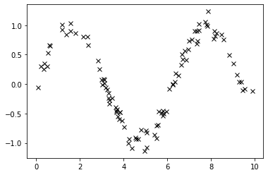
For this example, we create a synthetic dataset (noisy sine function):

def noisy_sin(x):
    return tf.math.sin(x) + 0.1 * tf.random.normal(x.shape, dtype=default_float())


num_train_data, num_test_data = 100, 500

X = tf.random.uniform((num_train_data, 1), dtype=default_float()) * 10
Xtest = tf.random.uniform((num_test_data, 1), dtype=default_float()) * 10

Y = noisy_sin(X)
Ytest = noisy_sin(Xtest)

data = (X, Y)

plt.plot(X, Y, "xk")
plt.show()

2022-05-10 10:47:39.049294: W tensorflow/stream_executor/platform/default/dso_loader.cc:64] Could not load dynamic library 'libcuda.so.1'; dlerror: libcuda.so.1: cannot open shared object file: No such file or directory
2022-05-10 10:47:39.049334: W tensorflow/stream_executor/cuda/cuda_driver.cc:269] failed call to cuInit: UNKNOWN ERROR (303)
2022-05-10 10:47:39.049355: I tensorflow/stream_executor/cuda/cuda_diagnostics.cc:156] kernel driver does not appear to be running on this host (49c966262641): /proc/driver/nvidia/version does not exist
2022-05-10 10:47:39.049723: I tensorflow/core/platform/cpu_feature_guard.cc:151] This TensorFlow binary is optimized with oneAPI Deep Neural Network Library (oneDNN) to use the following CPU instructions in performance-critical operations:  AVX2 AVX512F FMA
To enable them in other operations, rebuild TensorFlow with the appropriate compiler flags.

Working with TensorFlow Datasets is an efficient way to rapidly shuffle, iterate, and batch from data. For prefetch size we use tf.data.experimental.AUTOTUNE as recommended by TensorFlow guidelines.

train_dataset = tf.data.Dataset.from_tensor_slices((X, Y))
test_dataset = tf.data.Dataset.from_tensor_slices((Xtest, Ytest))

batch_size = 32
num_features = 10
prefetch_size = tf.data.experimental.AUTOTUNE
shuffle_buffer_size = num_train_data // 2
num_batches_per_epoch = num_train_data // batch_size

original_train_dataset = train_dataset
train_dataset = (
    train_dataset.repeat()
    .prefetch(prefetch_size)
    .shuffle(buffer_size=shuffle_buffer_size)
    .batch(batch_size)
)

print(f"prefetch_size={prefetch_size}")
print(f"shuffle_buffer_size={shuffle_buffer_size}")
print(f"num_batches_per_epoch={num_batches_per_epoch}")

prefetch_size=-1
shuffle_buffer_size=50
num_batches_per_epoch=3

Define a GP model

In GPflow 2.0, we use tf.Module (or the very thin gpflow.base.Module wrapper) to build all our models, as well as their components (kernels, likelihoods, parameters, and so on).

kernel = gpflow.kernels.SquaredExponential(variance=2.0)
likelihood = gpflow.likelihoods.Gaussian()
inducing_variable = np.linspace(0, 10, num_features).reshape(-1, 1)

model = gpflow.models.SVGP(
    kernel=kernel, likelihood=likelihood, inducing_variable=inducing_variable
)

You can set a module (or a particular parameter) to be non-trainable using the auxiliary method set_trainable(module, False):

from gpflow import set_trainable

set_trainable(likelihood, False)
set_trainable(kernel.variance, False)

set_trainable(likelihood, True)
set_trainable(kernel.variance, True)

2022-05-10 10:47:39.334370: W tensorflow/python/util/util.cc:368] Sets are not currently considered sequences, but this may change in the future, so consider avoiding using them.

We can use param.assign(value) to assign a value to a parameter:

kernel.lengthscales.assign(0.5)

<tf.Variable 'UnreadVariable' shape=() dtype=float64, numpy=-0.43275212956718856>

All these changes are reflected when we use print_summary(model) to print a detailed summary of the model. By default the output is displayed in a minimalistic and simple table.

from gpflow.utilities import print_summary

print_summary(model)  # same as print_summary(model, fmt="fancy_table")

╒══════════════════════════╤═══════════╤══════════════════╤═════════╤═════════════╤═════════════╤═════════╤══════════════════╕
│ name                     │ class     │ transform        │ prior   │ trainable   │ shape       │ dtype   │ value            │
╞══════════════════════════╪═══════════╪══════════════════╪═════════╪═════════════╪═════════════╪═════════╪══════════════════╡
│ SVGP.kernel.variance     │ Parameter │ Softplus         │         │ True        │ ()          │ float64 │ 2.0              │
├──────────────────────────┼───────────┼──────────────────┼─────────┼─────────────┼─────────────┼─────────┼──────────────────┤
│ SVGP.kernel.lengthscales │ Parameter │ Softplus         │         │ True        │ ()          │ float64 │ 0.5              │
├──────────────────────────┼───────────┼──────────────────┼─────────┼─────────────┼─────────────┼─────────┼──────────────────┤
│ SVGP.likelihood.variance │ Parameter │ Softplus + Shift │         │ True        │ ()          │ float64 │ 1.0              │
├──────────────────────────┼───────────┼──────────────────┼─────────┼─────────────┼─────────────┼─────────┼──────────────────┤
│ SVGP.inducing_variable.Z │ Parameter │ Identity         │         │ True        │ (10, 1)     │ float64 │ [[0....          │
├──────────────────────────┼───────────┼──────────────────┼─────────┼─────────────┼─────────────┼─────────┼──────────────────┤
│ SVGP.q_mu                │ Parameter │ Identity         │         │ True        │ (10, 1)     │ float64 │ [[0....          │
├──────────────────────────┼───────────┼──────────────────┼─────────┼─────────────┼─────────────┼─────────┼──────────────────┤
│ SVGP.q_sqrt              │ Parameter │ FillTriangular   │         │ True        │ (1, 10, 10) │ float64 │ [[[1., 0., 0.... │
╘══════════════════════════╧═══════════╧══════════════════╧═════════╧═════════════╧═════════════╧═════════╧══════════════════╛

We can change default printing so that it will look nicer in our notebook:

gpflow.config.set_default_summary_fmt("notebook")

print_summary(model)  # same as print_summary(model, fmt="notebook")

name	class	transform	prior	trainable	shape	dtype	value
SVGP.kernel.variance	Parameter	Softplus		True	()	float64	2.0
SVGP.kernel.lengthscales	Parameter	Softplus		True	()	float64	0.5
SVGP.likelihood.variance	Parameter	Softplus + Shift		True	()	float64	1.0
SVGP.inducing_variable.Z	Parameter	Identity		True	(10, 1)	float64	[[0....
SVGP.q_mu	Parameter	Identity		True	(10, 1)	float64	[[0....
SVGP.q_sqrt	Parameter	FillTriangular		True	(1, 10, 10)	float64	[[[1., 0., 0....

Jupyter notebooks also format GPflow classes (that are subclasses of gpflow.base.Module) in the same nice way when at the end of a cell (this is independent of the default_summary_fmt):

model

<gpflow.models.svgp.SVGP object at 0x7f872335a9b0>

name	class	transform	prior	trainable	shape	dtype	value
SVGP.kernel.variance	Parameter	Softplus		True	()	float64	2.0
SVGP.kernel.lengthscales	Parameter	Softplus		True	()	float64	0.5
SVGP.likelihood.variance	Parameter	Softplus + Shift		True	()	float64	1.0
SVGP.inducing_variable.Z	Parameter	Identity		True	(10, 1)	float64	[[0....
SVGP.q_mu	Parameter	Identity		True	(10, 1)	float64	[[0....
SVGP.q_sqrt	Parameter	FillTriangular		True	(1, 10, 10)	float64	[[[1., 0., 0....

Training using training_loss and training_loss_closure

GPflow models come with training_loss and training_loss_closure methods to make it easy to train your models. There is a slight difference between models that own their own data (most of them, e.g. GPR, VGP, …) and models that do not own the data (SVGP).

Model-internal data

For models that own their own data (inheriting from InternalDataTrainingLossMixin), data is provided at model construction time. In this case, model.training_loss does not take any arguments, and can be directly passed to an optimizer’s minimize() method:

vgp_model = gpflow.models.VGP(data, kernel, likelihood)
optimizer = tf.optimizers.Adam()
optimizer.minimize(
    vgp_model.training_loss, vgp_model.trainable_variables
)  # Note: this does a single step
# In practice, you will need to call minimize() many times, this will be further discussed below.

<tf.Variable 'UnreadVariable' shape=() dtype=int64, numpy=1>

This also works for the Scipy optimizer, though it will do the full optimization on a single call to minimize():

optimizer = gpflow.optimizers.Scipy()
optimizer.minimize(
    vgp_model.training_loss, vgp_model.trainable_variables, options=dict(maxiter=ci_niter(1000))
)

      fun: -67.28073919779587
 hess_inv: <5153x5153 LbfgsInvHessProduct with dtype=float64>
      jac: array([ 0.02205416, -0.02431949, -0.03372514, ..., -0.09714327,
        0.0029311 , -0.00230844])
  message: 'CONVERGENCE: REL_REDUCTION_OF_F_<=_FACTR*EPSMCH'
     nfev: 625
      nit: 581
     njev: 625
   status: 0
  success: True
        x: array([-0.19111145,  1.64416575,  0.0251442 , ...,  1.71382598,
        0.77107675, -4.65256621])

You can obtain a compiled version using training_loss_closure, whose compile argument is True by default:

vgp_model.training_loss_closure()  # compiled
vgp_model.training_loss_closure(compile=True)  # compiled
vgp_model.training_loss_closure(compile=False)  # uncompiled, same as vgp_model.training_loss

<bound method InternalDataTrainingLossMixin.training_loss of <gpflow.models.vgp.VGP object at 0x7f87233c6320>>

External data

The SVGP model inherits from ExternalDataTrainingLossMixin and expects the data to be passed to training_loss(). For SVGP as for the other regression models, data is a two-tuple of (X, Y), where X is an array/tensor with shape (num_data, input_dim) and Y is an array/tensor with shape (num_data, output_dim):

assert isinstance(model, gpflow.models.SVGP)
model.training_loss(data)

<tf.Tensor: shape=(), dtype=float64, numpy=8136.770384692683>

To make optimizing it easy, it has a training_loss_closure() method, that takes the data and returns a closure that computes the training loss on this data:

optimizer = tf.optimizers.Adam()
training_loss = model.training_loss_closure(
    data
)  # We save the compiled closure in a variable so as not to re-compile it each step
optimizer.minimize(training_loss, model.trainable_variables)  # Note that this does a single step

<tf.Variable 'UnreadVariable' shape=() dtype=int64, numpy=1>

SVGP can handle mini-batching, and an iterator from a batched tf.data.Dataset can be passed to the model’s training_loss_closure():

batch_size = 5
batched_dataset = tf.data.Dataset.from_tensor_slices(data).batch(batch_size)
training_loss = model.training_loss_closure(iter(batched_dataset))

optimizer.minimize(training_loss, model.trainable_variables)  # Note that this does a single step

<tf.Variable 'UnreadVariable' shape=() dtype=int64, numpy=2>

As previously, training_loss_closure takes an optional compile argument for tf.function compilation (True by default).

Training using Gradient Tapes

For a more elaborate example of a gradient update we can define an optimization_step that explicitly computes and applies gradients to the model. In TensorFlow 2, we can optimize (trainable) model parameters with TensorFlow optimizers using tf.GradientTape. In this simple example, we perform one gradient update of the Adam optimizer to minimize the training_loss (in this case the negative ELBO) of our model. The optimization_step can (and should) be wrapped in tf.function to be compiled to a graph if executing it many times.

def optimization_step(model: gpflow.models.SVGP, batch: Tuple[tf.Tensor, tf.Tensor]):
    with tf.GradientTape(watch_accessed_variables=False) as tape:
        tape.watch(model.trainable_variables)
        loss = model.training_loss(batch)
    grads = tape.gradient(loss, model.trainable_variables)
    optimizer.apply_gradients(zip(grads, model.trainable_variables))
    return loss

We can use the functionality of TensorFlow Datasets to define a simple training loop that iterates over batches of the training dataset:

def simple_training_loop(model: gpflow.models.SVGP, epochs: int = 1, logging_epoch_freq: int = 10):
    tf_optimization_step = tf.function(optimization_step)

    batches = iter(train_dataset)
    for epoch in range(epochs):
        for _ in range(ci_niter(num_batches_per_epoch)):
            tf_optimization_step(model, next(batches))

        epoch_id = epoch + 1
        if epoch_id % logging_epoch_freq == 0:
            tf.print(f"Epoch {epoch_id}: ELBO (train) {model.elbo(data)}")

simple_training_loop(model, epochs=10, logging_epoch_freq=2)

Epoch 2: ELBO (train) -7867.830422893827
Epoch 4: ELBO (train) -7665.490349558447
Epoch 6: ELBO (train) -7460.929343242079
Epoch 8: ELBO (train) -7258.373896232915
Epoch 10: ELBO (train) -7059.201134038565

Monitoring

gpflow.monitor provides a thin wrapper on top of tf.summary that makes it easy to monitor the training procedure. For a more detailed tutorial see the monitoring notebook.

from gpflow.monitor import (
    ImageToTensorBoard,
    ModelToTensorBoard,
    ExecuteCallback,
    Monitor,
    MonitorTaskGroup,
    ScalarToTensorBoard,
)


samples_input = np.linspace(0, 10, 100).reshape(-1, 1)


def plot_model(fig, ax):
    tf.print("Plotting...")
    mean, var = model.predict_f(samples_input)
    num_samples = 10
    samples = model.predict_f_samples(samples_input, num_samples)
    ax.plot(samples_input, mean, "C0", lw=2)
    ax.fill_between(
        samples_input[:, 0],
        mean[:, 0] - 1.96 * np.sqrt(var[:, 0]),
        mean[:, 0] + 1.96 * np.sqrt(var[:, 0]),
        color="C0",
        alpha=0.2,
    )
    ax.plot(X, Y, "kx")
    ax.plot(samples_input, samples[:, :, 0].numpy().T, "C0", linewidth=0.5)
    ax.set_ylim(-2.0, +2.0)
    ax.set_xlim(0, 10)


def print_cb(epoch_id=None, data=None):
    tf.print(f"Epoch {epoch_id}: ELBO (train)", model.elbo(data))


def elbo_cb(data=None, **_):
    return model.elbo(data)


output_logdir = enumerated_logdir()

model_task = ModelToTensorBoard(output_logdir, model)
elbo_task = ScalarToTensorBoard(output_logdir, elbo_cb, "elbo")
print_task = ExecuteCallback(callback=print_cb)

# We group these tasks and specify a period of `100` steps for them
fast_tasks = MonitorTaskGroup([model_task, elbo_task, print_task], period=100)

# We also want to see the model's fit during the optimisation
image_task = ImageToTensorBoard(output_logdir, plot_model, "samples_image")

# We typically don't want to plot too frequently during optimisation,
# which is why we specify a larger period for this task.
slow_taks = MonitorTaskGroup(image_task, period=500)
monitor = Monitor(fast_tasks, slow_taks)


def monitored_training_loop(epochs: int):
    tf_optimization_step = tf.function(optimization_step)

    batches = iter(train_dataset)

    for epoch in range(epochs):
        for _ in range(ci_niter(num_batches_per_epoch)):
            batch = next(batches)
            tf_optimization_step(model, batch)

        epoch_id = epoch + 1
        monitor(epoch, epoch_id=epoch_id, data=data)

NOTE: for optimal performance it is recommended to wrap the monitoring inside tf.function. This is detailed in the monitoring notebook.

model = gpflow.models.SVGP(
    kernel=kernel, likelihood=likelihood, inducing_variable=inducing_variable
)

monitored_training_loop(epochs=1000)

Epoch 1: ELBO (train) -7731.9489680942825
Plotting...
Epoch 101: ELBO (train) -2010.7499082553445
Epoch 201: ELBO (train) -835.84744685466865
Epoch 301: ELBO (train) -367.42098905310218
Epoch 401: ELBO (train) -154.340468263508
Epoch 501: ELBO (train) -52.994674241349458
Plotting...
Epoch 601: ELBO (train) -6.7676147819403587
Epoch 701: ELBO (train) 15.159145114828341
Epoch 801: ELBO (train) 27.205927858698992
Epoch 901: ELBO (train) 34.817422699172191

Then, we can use TensorBoard to examine the training procedure in more detail

# %tensorboard --logdir "{output_logdir}"

Saving and loading models

Checkpointing

With the help of tf.train.CheckpointManager and tf.train.Checkpoint, we can checkpoint the model throughout the training procedure. Let’s start with a simple example using checkpointing to save and load a tf.Variable:

initial_value = 1.2
a = tf.Variable(initial_value)

Create Checkpoint object:

ckpt = tf.train.Checkpoint(a=a)
manager = tf.train.CheckpointManager(ckpt, output_logdir, max_to_keep=3)

Save the variable a and change its value right after:

manager.save()
_ = a.assign(0.33)

Now we can restore the old variable value:

print(f"Current value of variable a: {a.numpy():0.3f}")

ckpt.restore(manager.latest_checkpoint)

print(f"Value of variable a after restore: {a.numpy():0.3f}")

Current value of variable a: 0.330
Value of variable a after restore: 1.200

In the example below, we modify a simple training loop to save the model every 100 epochs using the CheckpointManager.

model = gpflow.models.SVGP(
    kernel=kernel, likelihood=likelihood, inducing_variable=inducing_variable
)


def checkpointing_training_loop(
    model: gpflow.models.SVGP,
    batch_size: int,
    epochs: int,
    manager: tf.train.CheckpointManager,
    logging_epoch_freq: int = 100,
    epoch_var: Optional[tf.Variable] = None,
    step_var: Optional[tf.Variable] = None,
):
    tf_optimization_step = tf.function(optimization_step)

    batches = iter(train_dataset)

    for epoch in range(epochs):
        for step in range(ci_niter(num_batches_per_epoch)):
            tf_optimization_step(model, next(batches))
            if step_var is not None:
                step_var.assign(epoch * num_batches_per_epoch + step + 1)
        if epoch_var is not None:
            epoch_var.assign(epoch + 1)

        epoch_id = epoch + 1
        if epoch_id % logging_epoch_freq == 0:
            ckpt_path = manager.save()
            tf.print(f"Epoch {epoch_id}: ELBO (train) {model.elbo(data)}, saved at {ckpt_path}")

step_var = tf.Variable(1, dtype=tf.int32, trainable=False)
epoch_var = tf.Variable(1, dtype=tf.int32, trainable=False)
ckpt = tf.train.Checkpoint(model=model, step=step_var, epoch=epoch_var)
manager = tf.train.CheckpointManager(ckpt, output_logdir, max_to_keep=5)

print(f"Checkpoint folder path at: {output_logdir}")

checkpointing_training_loop(
    model,
    batch_size=batch_size,
    epochs=1000,
    manager=manager,
    epoch_var=epoch_var,
    step_var=step_var,
)

Checkpoint folder path at: /tmp/tensorboard/0
Epoch 100: ELBO (train) -147.83170413800735, saved at /tmp/tensorboard/0/ckpt-1
Epoch 200: ELBO (train) -7.956366143554943, saved at /tmp/tensorboard/0/ckpt-2
Epoch 300: ELBO (train) 24.97523975304129, saved at /tmp/tensorboard/0/ckpt-3
Epoch 400: ELBO (train) 36.85047959776172, saved at /tmp/tensorboard/0/ckpt-4
Epoch 500: ELBO (train) 42.18711351764152, saved at /tmp/tensorboard/0/ckpt-5
Epoch 600: ELBO (train) 45.088055848816964, saved at /tmp/tensorboard/0/ckpt-6
Epoch 700: ELBO (train) 46.9296278356626, saved at /tmp/tensorboard/0/ckpt-7
Epoch 800: ELBO (train) 48.25321201790865, saved at /tmp/tensorboard/0/ckpt-8
Epoch 900: ELBO (train) 49.30001561412369, saved at /tmp/tensorboard/0/ckpt-9
Epoch 1000: ELBO (train) 50.19449339619858, saved at /tmp/tensorboard/0/ckpt-10

After the models have been saved, we can restore them using tf.train.Checkpoint.restore and assert that their performance corresponds to that logged during training.

for i, recorded_checkpoint in enumerate(manager.checkpoints):
    ckpt.restore(recorded_checkpoint)
    print(
        f"{i} restored model from epoch {int(epoch_var)} [step:{int(step_var)}] : ELBO training set {model.elbo(data)}"
    )

0 restored model from epoch 600 [step:1800] : ELBO training set 45.088055848816964
1 restored model from epoch 700 [step:2100] : ELBO training set 46.9296278356626
2 restored model from epoch 800 [step:2400] : ELBO training set 48.25321201790865
3 restored model from epoch 900 [step:2700] : ELBO training set 49.30001561412369
4 restored model from epoch 1000 [step:3000] : ELBO training set 50.19449339619858

Copying (hyper)parameter values between models

It is easy to interact with the set of all parameters of a model or a subcomponent programmatically.

The following returns a dictionary of all parameters within

model = gpflow.models.SGPR(data, kernel=kernel, inducing_variable=inducing_variable)

gpflow.utilities.parameter_dict(model)

{'.kernel.variance': <Parameter: name=softplus, dtype=float64, shape=[], fn="softplus", numpy=0.8828930568889072>,
 '.kernel.lengthscales': <Parameter: name=softplus, dtype=float64, shape=[], fn="softplus", numpy=1.6777316501617014>,
 '.likelihood.variance': <Parameter: name=chain_of_shift_of_softplus, dtype=float64, shape=[], fn="chain_of_shift_of_softplus", numpy=1.0>,
 '.inducing_variable.Z': <Parameter: name=identity, dtype=float64, shape=[10, 1], fn="identity", numpy=
 array([[ 0.        ],
        [ 1.11111111],
        [ 2.22222222],
        [ 3.33333333],
        [ 4.44444444],
        [ 5.55555556],
        [ 6.66666667],
        [ 7.77777778],
        [ 8.88888889],
        [10.        ]])>}

Such a dictionary can be assigned back to this model (or another model with the same tree of parameters) as follows:

params = gpflow.utilities.parameter_dict(model)
gpflow.utilities.multiple_assign(model, params)

TensorFlow saved_model

In order to save the model we need to explicitly store the tf.function-compiled functions that we wish to export:

model.predict_f_compiled = tf.function(
    model.predict_f, input_signature=[tf.TensorSpec(shape=[None, 1], dtype=tf.float64)]
)

We also save the original prediction for later comparison. Here samples_input needs to be a tensor so that tf.function will compile a single graph:

samples_input = tf.convert_to_tensor(samples_input, dtype=default_float())
original_result = model.predict_f_compiled(samples_input)

Let’s save the model:

save_dir = str(pathlib.Path(tempfile.gettempdir()))
tf.saved_model.save(model, save_dir)

WARNING:absl:Function `predict_f` contains input name(s) Xnew with unsupported characters which will be renamed to xnew in the SavedModel.

WARNING:tensorflow:From /home/circleci/project/.venv/lib/python3.10/site-packages/tensorflow/python/training/tracking/autotrackable.py:90: Bijector.has_static_min_event_ndims (from tensorflow_probability.python.bijectors.bijector) is deprecated and will be removed after 2021-08-01.
Instructions for updating:
`min_event_ndims` is now static for all bijectors; this property is no longer needed.

WARNING:tensorflow:From /home/circleci/project/.venv/lib/python3.10/site-packages/tensorflow/python/training/tracking/autotrackable.py:90: Bijector.has_static_min_event_ndims (from tensorflow_probability.python.bijectors.bijector) is deprecated and will be removed after 2021-08-01.
Instructions for updating:
`min_event_ndims` is now static for all bijectors; this property is no longer needed.

INFO:tensorflow:Assets written to: /tmp/assets

INFO:tensorflow:Assets written to: /tmp/assets

We can load the module back as a new instance and compare the prediction results:

loaded_model = tf.saved_model.load(save_dir)
loaded_result = loaded_model.predict_f_compiled(samples_input)

np.testing.assert_array_equal(loaded_result, original_result)

User config update

In this notebook, we used a lot gpflow.config methods for setting and getting default attributes from global configuration. However, GPflow provides a way for local config modification without updating values in global. As you can see below, using gpflow.config.as_context replaces temporarily global config with your instance. At creation time, custom config instance uses standard values from the global config:

user_config = gpflow.config.Config(float=tf.float32, positive_bijector="exp")

user_str = "User config\t"
global_str = "Global config\t"

with gpflow.config.as_context(user_config):
    print(f"{user_str} gpflow.config.default_float = {gpflow.config.default_float()}")
    print(
        f"{user_str} gpflow.config.positive_bijector = {gpflow.config.default_positive_bijector()}"
    )

print(f"{global_str} gpflow.config.default_float = {gpflow.config.default_float()}")
print(f"{global_str} gpflow.config.positive_bijector = {gpflow.config.default_positive_bijector()}")

User config      gpflow.config.default_float = <dtype: 'float32'>
User config      gpflow.config.positive_bijector = exp
Global config    gpflow.config.default_float = <class 'numpy.float64'>
Global config    gpflow.config.positive_bijector = softplus

with gpflow.config.as_context(user_config):
    p = gpflow.Parameter(1.1, transform=gpflow.utilities.positive())
    print(f"{user_str}{p}")

p = gpflow.Parameter(1.1, transform=gpflow.utilities.positive())
print(f"{global_str}{p}")

User config     <Parameter: name=exp, dtype=float32, shape=[], fn="exp", numpy=1.1>
Global config   <Parameter: name=softplus, dtype=float64, shape=[], fn="softplus", numpy=1.1>