Basic Usage with GPR#
In this chapter we will go over the most basic concepts you will need to understand to use GPflow. We will train a simple model on some simple data; and demonstrate how to use the model to make predictions, and how to plot the results.
If your use-case is sufficiently simple, this chapter may be all you need to use
Imports#
These are the imports we’ll be assuming below:
[1]:
import matplotlib.pyplot as plt
import numpy as np

import gpflow
Meet \(f\) and \(Y\)#
In GPflow we usually assume our data is generated by a process:
\begin{equation} Y_i = f(X_i) + \varepsilon_i \,, \quad \varepsilon_i \sim \mathcal{N}(0, \sigma^2). \end{equation}
So we have some \(X\) values, that are pushed through some deterministic function \(f\), but we do not observe \(f(X)\) directly. Instead we get noisy observations — \(\varepsilon\) is some noise that is added before we observe \(Y\).
Usually we’ll either be interested in trying to recover \(f\) from our noisy observations, or trying to predict new values of \(Y\).
Notice that we have two sources of uncertainty here:
We have uncertainty about \(f\) which we get because we cannot learn \(f\) perfectly from a limited amount of noisy data. The more data we observe the smaller this uncertainty will be. (This is known as epistemic uncertainty.)
We have uncertainty about \(Y\) because of our noisy observations. No matter how much data we collect this will never become smaller, because this is an effect of the process we’re observing. (This is known as aleatoric uncertainty.)
It is important to understand the difference between \(f\) and \(Y\) to understand GPflow.
Minimal model#
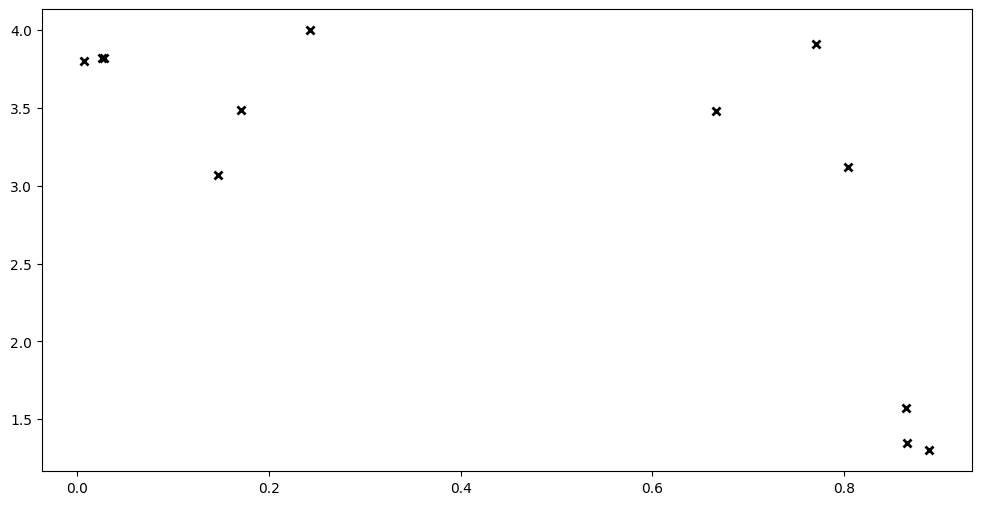
Let’s model some data. Below we have some variables X and Y, both of which are NumPy arrays, with shapes \(N \times D\) and \(N \times P\) respectively. \(N\) is the number of rows of data. \(D\) is the number of input dimensions, and \(P\) is the number of output dimensions. We set both \(D=1\) and \(P=1\) to keep things simple.
[2]:
X = np.array(
    [
        [0.865], [0.666], [0.804], [0.771], [0.147], [0.866], [0.007], [0.026],
        [0.171], [0.889], [0.243], [0.028],
    ]
)
Y = np.array(
    [
        [1.57], [3.48], [3.12], [3.91], [3.07], [1.35], [3.80], [3.82], [3.49],
        [1.30], [4.00], [3.82],
    ]
)

plt.plot(X, Y, "kx", mew=2)
To model this in GPflow, we first have to create a model:
[3]:
model = gpflow.models.GPR(
    (X, Y),
    kernel=gpflow.kernels.SquaredExponential(),
)
Here we use a GPR model with an SquaredExponential kernel. We’ll go into more details about what that means in other chapters, but these are sensible defaults for small, simple problems.
Next we need to train the model:
[4]:
opt = gpflow.optimizers.Scipy()
opt.minimize(model.training_loss, model.trainable_variables)
Now we can use the model to predict values of \(f\) and \(Y\) at new values of \(X\).
The main methods for making predictions are model.predict_f and model.predict_y. model.predict_f returns the mean and variance (uncertainty) the function \(f\), while model.predict_y returns the mean and variance (uncertainty) of \(Y\) — that is \(f\) plus the noise.
So, if we want to know what the model thinks \(f\) might be at 0.5 we do:
[5]:
Xnew = np.array([[0.5]])
model.predict_f(Xnew)
[5]:
(<tf.Tensor: shape=(1, 1), dtype=float64, numpy=array([[4.28009566]])>,
 <tf.Tensor: shape=(1, 1), dtype=float64, numpy=array([[0.30584767]])>)
And if we want to predict \(Y\):
[6]:
model.predict_y(Xnew)
[6]:
(<tf.Tensor: shape=(1, 1), dtype=float64, numpy=array([[4.28009566]])>,
 <tf.Tensor: shape=(1, 1), dtype=float64, numpy=array([[0.54585965]])>)
Notice how the predicted \(f\) and \(Y\) have the same mean, but \(Y\) has a larger variance. This is because the variance of \(f\) is only the uncertainty of \(f\), while the variance of \(Y\) is both the uncertainty of \(f\) and the extra noise.
Plotting the model#
Now, lets predict \(f\) and \(Y\) for a range of \(X\)s and make a pretty plot of it.
First we generate some test points for the prediction:
[7]:
Xplot = np.linspace(-0.1, 1.1, 100)[:, None]
Then we predict the \(f\) and \(Y\) values:
[8]:
f_mean, f_var = model.predict_f(Xplot, full_cov=False)
y_mean, y_var = model.predict_y(Xplot)
We compute the 95% confidence interval of \(f\) and \(Y\). This math is based on the distribution of \(f\) and \(Y\) being gaussian:
[9]:
f_lower = f_mean - 1.96 * np.sqrt(f_var)
f_upper = f_mean + 1.96 * np.sqrt(f_var)
y_lower = y_mean - 1.96 * np.sqrt(y_var)
y_upper = y_mean + 1.96 * np.sqrt(y_var)
Finally we actually plot our values:
[10]:
plt.plot(X, Y, "kx", mew=2, label="input data")
plt.plot(Xplot, f_mean, "-", color="C0", label="mean")
plt.plot(Xplot, f_lower, "--", color="C0", label="f 95% confidence")
plt.plot(Xplot, f_upper, "--", color="C0")
plt.fill_between(
    Xplot[:, 0], f_lower[:, 0], f_upper[:, 0], color="C0", alpha=0.1
)
plt.plot(Xplot, y_lower, ".", color="C0", label="Y 95% confidence")
plt.plot(Xplot, y_upper, ".", color="C0")
plt.fill_between(
    Xplot[:, 0], y_lower[:, 0], y_upper[:, 0], color="C0", alpha=0.1
)
plt.legend()
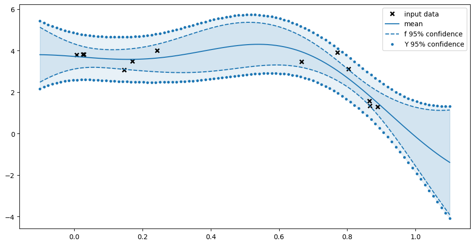
Notice how the confidence of \(f\) is greater when you’re further away from our data, and smaller near the data. Notice also how we’re more certain about \(f\) than about \(Y\); sometimes we’re even certain that \(f\) lies away from a data point.
Marginal variance vs full covariance#
As mentioned above \(f\) is a function, and we expect it to be, more or less, smooth. So if \(x_1\) and \(x_2\) are near each other, we expect \(f(x_1)\) and \(f(x_2)\) to be near each other as well. In Gaussian Processes we encode the information about how nearby values of \(x\) are similar with a covariance matrix.
If we call predict_f(..., full_cov=False) like we did above, when we plotted the model, predict_f will return a \(N \times P\) mean vector and a \(N \times P\) marginal variance vector. The marginal variance vector only tells us about our uncertainty at each point individually, and does not tell us anything about how the points relate to each other. Often the marginal variance vector is all you need, and it is faster to compute than the full covariance. False is the default
value for full_cov.
[11]:
Xnew = np.array([[0.3], [0.5], [0.7]])
model.predict_f(Xnew, full_cov=False)
[11]:
(<tf.Tensor: shape=(3, 1), dtype=float64, numpy=
 array([[3.75907766],
        [4.28009566],
        [3.71506022]])>,
 <tf.Tensor: shape=(3, 1), dtype=float64, numpy=
 array([[0.17286964],
        [0.30584767],
        [0.11372553]])>)
If we call predict_f(..., full_cov=True) we will still get a \(N \times P\) mean vector, but instead of the marginal variance we will get a full \(P \times N \times N\) covariance matrix, which tells us the relationship between different values of \(x\).
[12]:
model.predict_f(Xnew, full_cov=True)
[12]:
(<tf.Tensor: shape=(3, 1), dtype=float64, numpy=
 array([[3.75907766],
        [4.28009566],
        [3.71506022]])>,
 <tf.Tensor: shape=(1, 3, 3), dtype=float64, numpy=
 array([[[0.17286964, 0.18033224, 0.04013752],
         [0.18033224, 0.30584767, 0.12780391],
         [0.04013752, 0.12780391, 0.11372553]]])>)
Technically the marginal variance vector we get with predict_f(..., full_cov=False) is just the diagonal of the full covariance matrix we get with predict_f(..., full_cov=True), but the former is faster to compute, so prefer that when possible.
What’s next?#
On this page we gave you a very quick overview of how a GPflow model is created, and how we can use it to make predictions. On the following pages we will go into details of different kind of GPflow models, how they are configured and, how they are trained.