Sanity checking when model behaviours should overlap

Many of the model classes in GPflow have overlapping behaviour in special cases. In this notebook, we fit some approximations to a model with a Gaussian likelihood, and make sure they’re all the same.

The models are: - GPR: Full Gaussian process regression.

• VGP: A Gaussian approximation with Variational Bayes. Approximating a Gaussian posterior with a Gaussian should be exact.

• SVGP: a sparse GP, with a Gaussian approximation. The inducing points are set to be at the data points, so again, should be exact.

• SVGP (with whitened representation): As above, but with a rotation applied to whiten the representation of the process.

• SGPR: A sparse GP with a collapsed posterior (Titsias 2009). Again, the inducing points are fixed to the data points.

• GPRFITC: The FITC approximation. Again, the inducing points are fixed to the data points.

In all cases the parameters are estimated by the method of maximum likelihood (or approximate maximum likelihood, as appropriate). The parameter estimates should all be the same.

import matplotlib.pyplot as plt
import numpy as np
import tensorflow as tf

import gpflow
from gpflow import set_trainable
from gpflow.ci_utils import reduce_in_tests
from gpflow.config import default_float
from gpflow.models import (
    maximum_log_likelihood_objective,
    training_loss_closure,
)

%matplotlib inline
plt.rcParams["figure.figsize"] = (12, 6)

2023-08-09 12:26:15.810520: W tensorflow/compiler/tf2tensorrt/utils/py_utils.cc:38] TF-TRT Warning: Could not find TensorRT

np.random.seed(0)
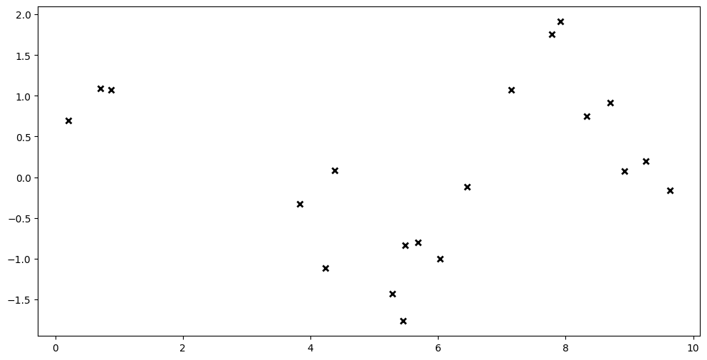
X = np.random.rand(20, 1) * 10
Y = np.sin(X) + 0.9 * np.cos(X * 1.6) + np.random.randn(*X.shape) * 0.4
Xtest = np.random.rand(10, 1) * 10
plt.plot(X, Y, "kx", mew=2)

data = (
    tf.convert_to_tensor(X, dtype=default_float()),
    tf.convert_to_tensor(Y, dtype=default_float()),
)
inducing_variable = tf.convert_to_tensor(X, dtype=default_float())

m1 = gpflow.models.GPR(data, kernel=gpflow.kernels.SquaredExponential())
m2 = gpflow.models.VGP(
    data,
    kernel=gpflow.kernels.SquaredExponential(),
    likelihood=gpflow.likelihoods.Gaussian(),
)
m3 = gpflow.models.SVGP(
    gpflow.kernels.SquaredExponential(),
    gpflow.likelihoods.Gaussian(),
    inducing_variable,
    q_diag=False,
)
set_trainable(m3.inducing_variable, False)

m4 = gpflow.models.SVGP(
    gpflow.kernels.SquaredExponential(),
    gpflow.likelihoods.Gaussian(),
    inducing_variable,
    q_diag=False,
    whiten=True,
)
set_trainable(m4.inducing_variable, False)

m5 = gpflow.models.SGPR(
    data,
    kernel=gpflow.kernels.SquaredExponential(),
    inducing_variable=inducing_variable,
)
set_trainable(m5.inducing_variable, False)

m6 = gpflow.models.GPRFITC(
    data,
    kernel=gpflow.kernels.SquaredExponential(),
    inducing_variable=inducing_variable,
)
set_trainable(m6.inducing_variable, False)

models = [m1, m2, m3, m4, m5, m6]

Now, we optimize the models. For GPR, SVGP, and GPRFITC, this simply optimizes the hyperparameters (since the inducing points are fixed). For the variational models, this jointly maximises the lower bound to the marginal likelihood (Evidence Lower Bound, ELBO) with respect to the variational parameters and the kernel and likelihood hyperparameters.

for m in models:
    opt = gpflow.optimizers.Scipy()
    loss_closure = training_loss_closure(m, data)
    opt.minimize(
        loss_closure,
        variables=m.trainable_variables,
        options=dict(maxiter=reduce_in_tests(1000)),
        compile=True,
    )

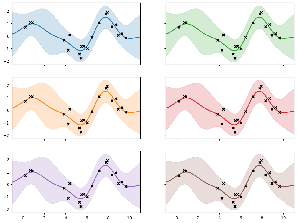
If everything worked as planned, the models should have the same:

• prediction functions

• log (marginal) likelihood

• kernel parameters

For the variational models, where we use a ELBO in place of the likelihood, the ELBO should be tight to the likelihood in the cases studied here.

def plot(m, color, ax):
    xx = np.linspace(-1, 11, 100)[:, None]
    mu, var = m.predict_y(xx)
    ax.plot(xx, mu, color, lw=2)
    ax.fill_between(
        xx[:, 0],
        mu[:, 0] - 2 * np.sqrt(var[:, 0]),
        mu[:, 0] + 2 * np.sqrt(var[:, 0]),
        color=color,
        alpha=0.2,
    )
    ax.plot(X, Y, "kx", mew=2)
    ax.set_xlim(-1, 11)


f, ax = plt.subplots(3, 2, sharex=True, sharey=True, figsize=(12, 9))
plot(m1, "C0", ax[0, 0])
plot(m2, "C1", ax[1, 0])
plot(m3, "C2", ax[0, 1])
plot(m4, "C3", ax[1, 1])
plot(m5, "C4", ax[2, 0])
plot(m6, "C5", ax[2, 1])

Here are the kernels and likelihoods, which show the fitted kernel parameters and noise variance:

for m in models:
    print(m.__class__.__name__)
    print(f"  kernel lengthscale  = {m.kernel.lengthscales.numpy():.5g}")
    print(f"  kernel variance     = {m.kernel.variance.numpy():.5}")
    print(f"  likelihood variance = {m.likelihood.variance.numpy():.5}")

GPR
  kernel lengthscale  = 1.0774
  kernel variance     = 0.82561
  likelihood variance = 0.16002
VGP
  kernel lengthscale  = 1.0773
  kernel variance     = 0.82546
  likelihood variance = 0.16002
SVGP
  kernel lengthscale  = 1.0774
  kernel variance     = 0.82549
  likelihood variance = 0.16003
SVGP
  kernel lengthscale  = 1.0774
  kernel variance     = 0.82549
  likelihood variance = 0.16003
SGPR
  kernel lengthscale  = 1.0774
  kernel variance     = 0.82561
  likelihood variance = 0.16002
GPRFITC
  kernel lengthscale  = 1.0774
  kernel variance     = 0.82561
  likelihood variance = 0.16002

Here are the likelihoods (or ELBOs):

for m in models:
    print(
        f"{m.__class__.__name__:30}  {maximum_log_likelihood_objective(m, data)}"
    )

GPR                             -18.83436136005674
VGP                             -18.834361541124224
SVGP                            -18.834400091469195
SVGP                            -18.834400091469195
SGPR                            -18.83439998906201
GPRFITC                         -18.834354780715604