Gaussian process regression with varying output noise

This notebook shows how to construct a Gaussian process model where different noise is assumed for different data points. The model is:

\begin{align} f(\cdot) &\sim \mathcal{GP}\big(0, k(\cdot, \cdot)\big) \\ y_i | f, x_i &\sim \mathcal N\big(y_i; f(x_i), \sigma^2_i\big) \end{align}

We’ll demonstrate three methods for specifying the data-point specific noise: * First we’ll show how to fit the noise variance to a simple function. * In the second demonstration we’ll assume that the data comes from two different groups and show how to learn separate noise variance for the groups. * Third we’ll assume you have multiple samples at each location \(x\) and show how to use the empirical variance.

import os
import warnings

warnings.simplefilter("ignore")
os.environ["TF_CPP_MIN_LOG_LEVEL"] = "3"

from typing import Optional, Tuple

import matplotlib.pyplot as plt
import numpy as np
import tensorflow as tf

import gpflow as gf
from gpflow.ci_utils import reduce_in_tests
from gpflow.experimental.check_shapes import inherit_check_shapes
from gpflow.utilities import print_summary

%matplotlib inline

gf.config.set_default_summary_fmt("notebook")

optimizer_config = dict(maxiter=reduce_in_tests(1000))
n_data = reduce_in_tests(300)
X_plot = np.linspace(0.0, 1.0, reduce_in_tests(101))[:, None]

To help us later we’ll first define a small function for plotting data with predictions:

def plot_distribution(
    X: gf.base.AnyNDArray,
    Y: gf.base.AnyNDArray,
    X_plot: Optional[gf.base.AnyNDArray] = None,
    mean_plot: Optional[gf.base.AnyNDArray] = None,
    var_plot: Optional[gf.base.AnyNDArray] = None,
    X_err: Optional[gf.base.AnyNDArray] = None,
    mean_err: Optional[gf.base.AnyNDArray] = None,
    var_err: Optional[gf.base.AnyNDArray] = None,
) -> None:
    plt.figure(figsize=(15, 5))

    X = X.squeeze(axis=-1)
    Y = Y.squeeze(axis=-1)
    plt.scatter(X, Y, color="gray", alpha=0.8)

    def get_confidence_bounds(
        mean: gf.base.AnyNDArray, var: gf.base.AnyNDArray
    ) -> Tuple[gf.base.AnyNDArray, gf.base.AnyNDArray]:
        std = np.sqrt(var)
        return mean - 1.96 * std, mean + 1.96 * std

    if X_plot is not None:
        assert mean_plot is not None
        assert var_plot is not None
        X_plot = X_plot.squeeze(axis=-1)
        mean_plot = mean_plot.squeeze(axis=-1)
        var_plot = var_plot.squeeze(axis=-1)
        lower_plot, upper_plot = get_confidence_bounds(mean_plot, var_plot)
        plt.fill_between(X_plot, lower_plot, upper_plot, color="silver", alpha=0.25)
        plt.plot(X_plot, lower_plot, color="silver")
        plt.plot(X_plot, upper_plot, color="silver")
        plt.plot(X_plot, mean_plot, color="black")

    if X_err is not None:
        assert mean_err is not None
        assert var_err is not None
        lower_err, upper_err = get_confidence_bounds(mean_err, var_err)
        plt.vlines(X_err, lower_err, upper_err, color="black")

    plt.xlim([0, 1])
    plt.show()

Demo 1: known noise variances

Generate data

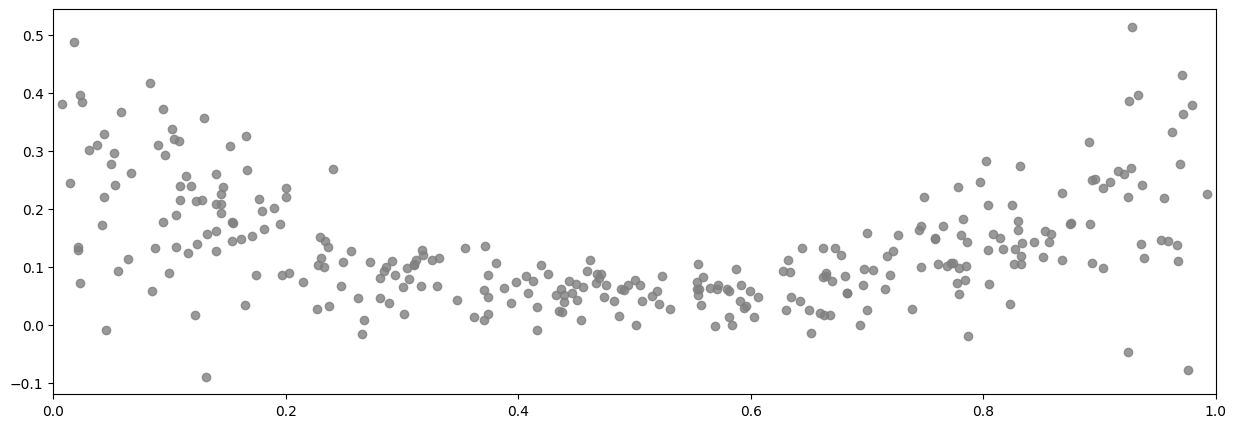
We create a utility function to generate synthetic data, including noise that varies amongst the data:

def generate_data() -> Tuple[gf.base.AnyNDArray, gf.base.AnyNDArray]:
    rng = np.random.default_rng(42)  # for reproducibility
    X = rng.uniform(0.0, 1.0, (n_data, 1))
    signal = (X - 0.5) ** 2 + 0.05
    noise_scale = 0.5 * signal
    noise = noise_scale * rng.standard_normal((n_data, 1))
    Y = signal + noise
    return X, Y


X, Y = generate_data()

The data alone looks like:

plot_distribution(X, Y)

Try a naive fit

If we try to fit a naive GPR model to this data, which assumes a single shared noise variance value for all data points - as specified by the likelihood variance parameter - we get:

model = gf.models.GPR(
    data=(X, Y),
    kernel=gf.kernels.SquaredExponential(),
)
gf.optimizers.Scipy().minimize(
    model.training_loss, model.trainable_variables, options=optimizer_config
)
print_summary(model)

name	class	transform	prior	trainable	shape	dtype	value
GPR.kernel.variance	Parameter	Softplus		True	()	float64	0.12365
GPR.kernel.lengthscales	Parameter	Softplus		True	()	float64	0.61646
GPR.likelihood.variance	Parameter	Softplus + Shift		True	()	float64	0.0057

mean, var = model.predict_y(X_plot)
plot_distribution(X, Y, X_plot, mean.numpy(), var.numpy())

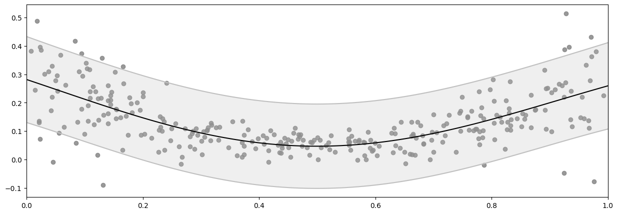
Notice how this naive model underestimates the noise near the center of the figure, but overestimates at for small and large values of x?

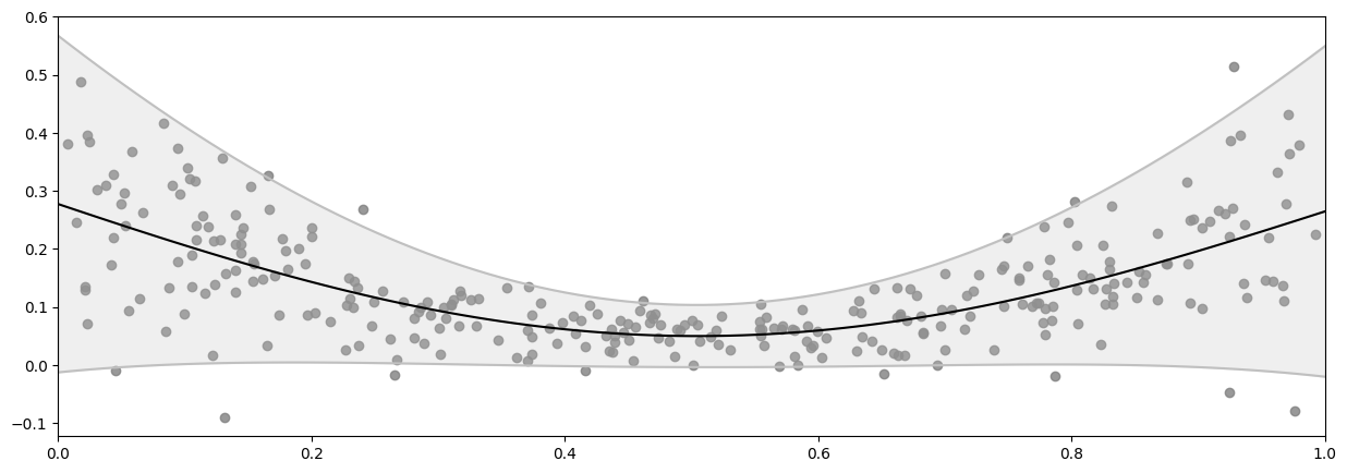
Fit a polynomial to the noise scale

To fit a model with varying noise, instead of using the default single shared noise variance, we can create a Gaussian Likelihood with an input dependent (polynomial) Function for the scale of the noise, then pass that likelihood to our model.

model = gf.models.GPR(
    data=(X, Y),
    kernel=gf.kernels.SquaredExponential(),
    likelihood=gf.likelihoods.Gaussian(scale=gf.functions.Polynomial(degree=2)),
)
gf.optimizers.Scipy().minimize(
    model.training_loss, model.trainable_variables, options=optimizer_config
)
print_summary(model)

name	class	transform	prior	trainable	shape	dtype	value
GPR.kernel.variance	Parameter	Softplus		True	()	float64	0.24138
GPR.kernel.lengthscales	Parameter	Softplus		True	()	float64	0.77092
GPR.likelihood.scale.w	Parameter	Identity		True	(1, 3)	float64	[[ 0.14643 -0.47433 0.47147]]

mean, var = model.predict_y(X_plot)
plot_distribution(X, Y, X_plot, mean.numpy(), var.numpy())

Demo 2: grouped noise variances

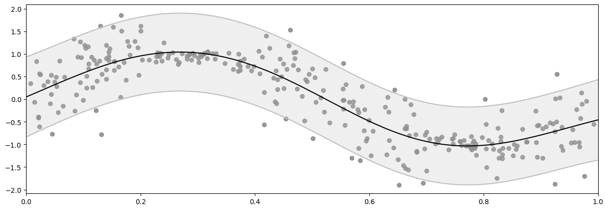
In this demo, we won’t assume that the noise variances is a function of \(x\), but we will assume that they’re known to be in two groups. This example represents a case where we might know that data has been collected by two instruments with different fidelity, but we do not know what those fidelities are.

Of course it would be straightforward to add more groups. We’ll stick with two for simplicity.

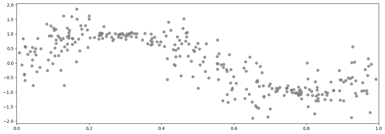
Generate data

def get_group(X: gf.base.AnyNDArray) -> gf.base.AnyNDArray:
    return np.where((((0.2 < X) & (X < 0.4)) | ((0.7 < X) & (X < 0.8))), 0, 1)


def generate_grouped_data() -> Tuple[gf.base.AnyNDArray, gf.base.AnyNDArray]:
    rng = np.random.default_rng(42)  # for reproducibility
    X = rng.uniform(0.0, 1.0, (n_data, 1))
    signal = np.sin(6 * X)
    noise_scale = 0.1 + 0.4 * get_group(X)
    noise = noise_scale * rng.standard_normal((n_data, 1))
    Y = signal + noise
    return X, Y


X, Y = generate_grouped_data()

And here’s a plot of the raw data:

plot_distribution(X, Y)

Fit a naive model

Again we’ll start by fitting a naive GPR, to demonstrate the problem.

model = gf.models.GPR(
    data=(X, Y),
    kernel=gf.kernels.SquaredExponential(),
)
gf.optimizers.Scipy().minimize(
    model.training_loss, model.trainable_variables, options=optimizer_config
)
print_summary(model)

name	class	transform	prior	trainable	shape	dtype	value
GPR.kernel.variance	Parameter	Softplus		True	()	float64	0.66418
GPR.kernel.lengthscales	Parameter	Softplus		True	()	float64	0.2537
GPR.likelihood.variance	Parameter	Softplus + Shift		True	()	float64	0.18977

mean, var = model.predict_y(X_plot)
plot_distribution(X, Y, X_plot, mean.numpy(), var.numpy())

Data structure

To model the different noise groups, we need to let the model know which group each data point belongs to. We’ll do that by appending a column with the group to the \(x\) data:

X_and_group = np.hstack([X, get_group(X)])
X_plot_and_group = np.hstack([X_plot, get_group(X_plot)])

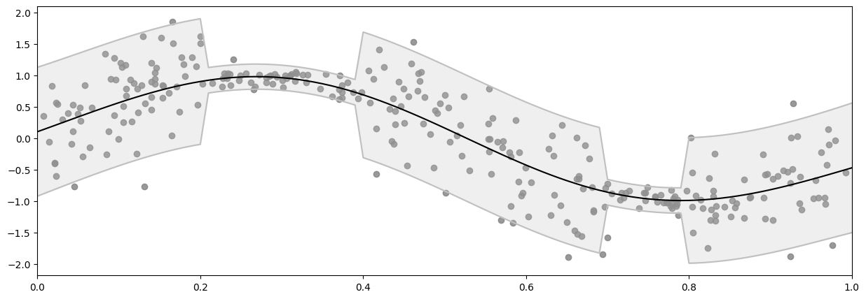
Use multiple functions for the noise variance

To model this we will create two noise variance functions, each of which are just a constant, and then switch between them depending on the group labels.

Notice that we initialize the constant functions to a positive value. They would have defaulted to 0.0, but that wouldn’t work for a variance, which must be strictly positive.

model = gf.models.GPR(
    data=(X_and_group, Y),
    kernel=gf.kernels.SquaredExponential(active_dims=[0]),
    likelihood=gf.likelihoods.Gaussian(
        variance=gf.functions.SwitchedFunction(
            [
                gf.functions.Constant(1.0),
                gf.functions.Constant(1.0),
            ]
        )
    ),
)
gf.optimizers.Scipy().minimize(
    model.training_loss, model.trainable_variables, options=optimizer_config
)
print_summary(model)

name	class	transform	prior	trainable	shape	dtype	value
GPR.kernel.variance	Parameter	Softplus		True	()	float64	0.81565
GPR.kernel.lengthscales	Parameter	Softplus		True	()	float64	0.30409
GPR.likelihood.variance.functions[0].c	Parameter	Identity		True	()	float64	0.01012
GPR.likelihood.variance.functions[1].c	Parameter	Identity		True	()	float64	0.25862

mean, var = model.predict_y(X_plot_and_group)
plot_distribution(X, Y, X_plot, mean.numpy(), var.numpy())

Demo 3: Empirical noise variance

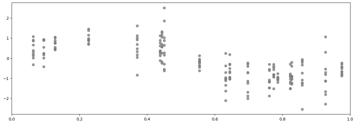
In this demo we will assume that you have multiple measurements at each \(x\) location, and want to use the empirical variance at each location.

Generate data

n_data = reduce_in_tests(20)
n_repeats = reduce_in_tests(10)


def generate_empiricial_noise_data() -> Tuple[gf.base.AnyNDArray, gf.base.AnyNDArray]:
    rng = np.random.default_rng(42)  # for reproducibility
    X = rng.uniform(0.0, 1.0, (n_data, 1))
    signal = np.sin(6 * X)
    noise_scale = rng.uniform(0.1, 1.0, (n_data, 1))
    noise = noise_scale * rng.standard_normal((n_data, n_repeats))
    Y = signal + noise
    return X, Y


X, Y = generate_empiricial_noise_data()
Y_mean = np.mean(Y, axis=-1, keepdims=True)
Y_var = np.var(Y, axis=-1, keepdims=True)

For the sake of plotting we’ll create flat lists of (x, y) pairs:

X_flat = np.broadcast_to(X, Y.shape).reshape((-1, 1))
Y_flat = Y.reshape((-1, 1))
plot_distribution(X_flat, Y_flat)

Data structure

Our GPs don’t like it when multiple data points occupy the same \(x\) location. So we’ll reduce this dataset to the means and the variances at each \(x\), and use a custom function to model inject the empirical variances into the model.

Y_mean = np.mean(Y, axis=-1, keepdims=True)

Fit a naive model

Again we’ll start by fitting a naive GPR, to demonstrate the problem.

Notice that this case is somewhat different from what we did above. Here we are not modelling \(Y\), but the mean of \(Y\), so the noise variance is not our uncertainty of \(Y\), but our uncertainty of the mean of \(Y\). Furthermore, while the naive model assumes a constant noise variance, the custom noise variance function we will develop below will only model the noise variance at the points where we have data, thus we cannot plot a continuous uncertainty. Instead, the shaded gray area is the confidence interval of \(f\), and we use vertical black lines to indicate the confidence interval of the \(Y\) mean.

model = gf.models.GPR(
    data=(X, Y_mean),
    kernel=gf.kernels.SquaredExponential(),
)
gf.optimizers.Scipy().minimize(
    model.training_loss, model.trainable_variables, options=optimizer_config
)
print_summary(model)

name	class	transform	prior	trainable	shape	dtype	value
GPR.kernel.variance	Parameter	Softplus		True	()	float64	0.5174
GPR.kernel.lengthscales	Parameter	Softplus		True	()	float64	0.24234
GPR.likelihood.variance	Parameter	Softplus + Shift		True	()	float64	0.02477

f_mean, f_var = model.predict_f(X_plot)
y_mean_mean, y_mean_var = model.predict_y(X)

plot_distribution(
    X_flat,
    Y_flat,
    X_plot,
    f_mean.numpy(),
    f_var.numpy(),
    X,
    y_mean_mean.numpy(),
    y_mean_var.numpy(),
)

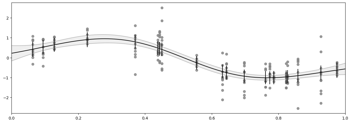
Create custom function for the noise variance

We’re modelling the Y_mean and its standard error is Y_var / n_repeats. We will create a simple function that ignores its input and returns these values as a constant. This will obviously only work for the X that corresponds to the Y we computed the variance of - that is good enough for model training, but notice that it will not allow us to use predict_y.

class FixedVarianceOfMean(gf.functions.Function):
    def __init__(self, Y: gf.base.AnyNDArray):
        n_repeats = Y.shape[-1]
        self.var_mean = np.var(Y, axis=-1, keepdims=True) / n_repeats

    @inherit_check_shapes
    def __call__(self, X: gf.base.TensorType) -> tf.Tensor:
        return self.var_mean

Now we can plug that into our model:

model = gf.models.GPR(
    data=(X, Y_mean),
    kernel=gf.kernels.SquaredExponential(active_dims=[0]),
    likelihood=gf.likelihoods.Gaussian(variance=FixedVarianceOfMean(Y)),
)
gf.optimizers.Scipy().minimize(
    model.training_loss, model.trainable_variables, options=optimizer_config
)
print_summary(model)

name	class	transform	prior	trainable	shape	dtype	value
GPR.kernel.variance	Parameter	Softplus		True	()	float64	0.60614
GPR.kernel.lengthscales	Parameter	Softplus		True	()	float64	0.26903

f_mean, f_var = model.predict_f(X_plot)
y_mean_mean, y_mean_var = model.predict_y(X)

plot_distribution(
    X_flat,
    Y_flat,
    X_plot,
    f_mean.numpy(),
    f_var.numpy(),
    X,
    y_mean_mean.numpy(),
    y_mean_var.numpy(),
)

You may notice that the data points fall outside our confidence interval. Again, this is because the confidence interval is for the mean of \(Y\), and not the \(Y\) points themselves.

Further reading

To model the variance using a second GP, see the Heteroskedastic regression notebook.