Mean Functions

In the previous chapter we talked about kernels. If you go back and look at the plots, you may notice that even in the plots without any data, where we just look at \(f\) samples, the \(f\) samples are kind of close to 0. Why is that? The kernels define what kinds of shape \(f\) can take, but not where the function is; a mean function defines where. In the section on kernels we didn’t specify a mean function, and the default mean function is constant 0, which explains why, by default, \(f\) samples will be close to 0.

As usual we will start with some necessary imports:

import matplotlib.pyplot as plt
import numpy as np
import tensorflow as tf
from check_shapes import inherit_check_shapes

import gpflow

And a helper function to visualise our models:

def plot_model(
    model: gpflow.models.GPModel,
    *,
    min_x: float,
    max_x: float,
    optimise: bool = True,
) -> None:
    _, ax = plt.subplots(nrows=1, ncols=1)

    if optimise:
        opt = gpflow.optimizers.Scipy()
        opt.minimize(model.training_loss, model.trainable_variables)

    Xplot = np.linspace(min_x, max_x, 300)[:, None]

    f_mean, f_var = model.predict_f(Xplot, full_cov=False)
    f_lower = f_mean - 1.96 * np.sqrt(f_var)
    f_upper = f_mean + 1.96 * np.sqrt(f_var)

    ax.hlines(0.0, min_x, max_x, colors="black", linestyles="dotted", alpha=0.3)
    ax.scatter(X, Y, color="black")
    (mean_line,) = ax.plot(Xplot, f_mean, "-")
    color = mean_line.get_color()
    ax.plot(Xplot, f_lower, lw=0.1, color=color)
    ax.plot(Xplot, f_upper, lw=0.1, color=color)
    ax.fill_between(
        Xplot[:, 0], f_lower[:, 0], f_upper[:, 0], color=color, alpha=0.1
    )

Mean reversion

Observe:

X = np.array([[0.0], [0.1], [0.2], [0.3], [0.4]])
Y = np.array([[2.0], [1.7], [1.6], [1.7], [2.0]])
model = gpflow.models.GPR((X, Y), kernel=gpflow.kernels.Matern32())
plot_model(model, min_x=-0.1, max_x=4.1)

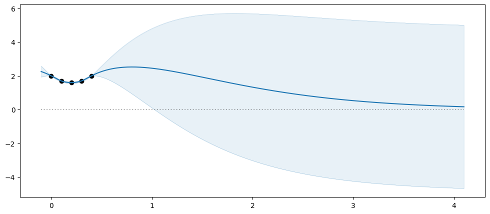
As we move away from the data our predictions converge towards 0. Basically, as we move away from the data, the model does not know what to predict, and will revert towards the mean function. This is called “mean reversion”, and this is the primary use case where having a reasonable mean function can help. In the areas where we have plenty of data, we don’t need a mean function.

Setting a mean function

Our models generally take a mean_function object that you can set to any instance of gpflow.functions.MeanFunction. See our API documentation for a full list of built-in mean functions.

In the above example I happen to know that our data is a quadratic function, so let us try setting our mean function to a 2nd degree polynomial:

model = gpflow.models.GPR(
    (X, Y),
    kernel=gpflow.kernels.Matern32(),
    mean_function=gpflow.functions.Polynomial(2),
)
plot_model(model, min_x=-0.1, max_x=4.1)

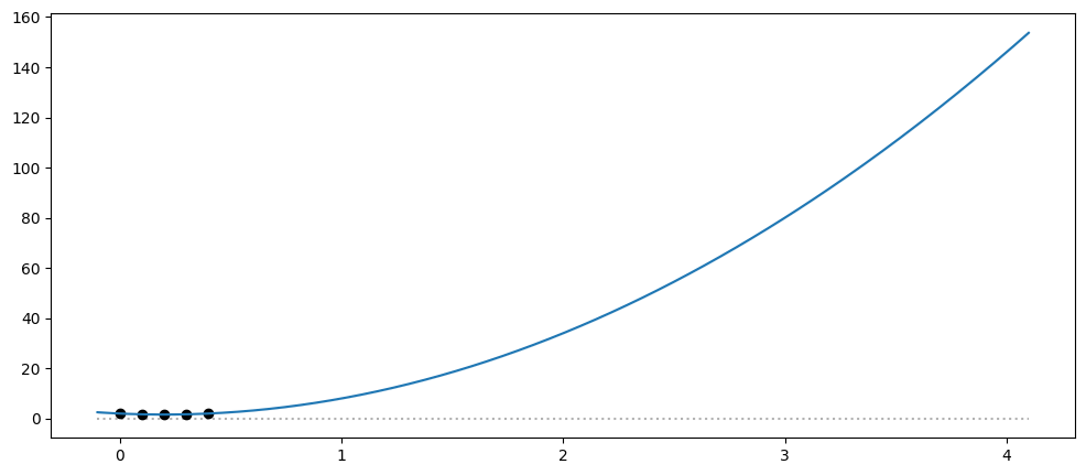
Our model now fits our mean function to the data without any noise, and happily extrapolates the quadratic function.

Interactions with the kernel

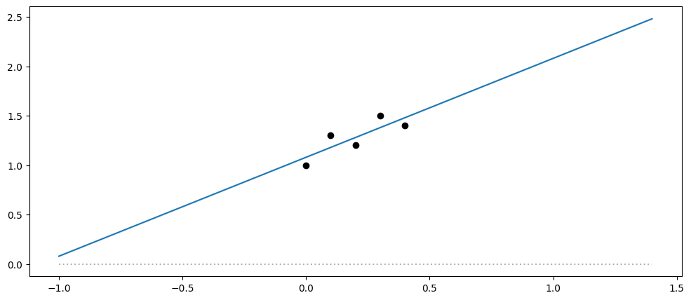
The shape of \(f\) relative to the mean function is determined by the kernel.

So, if we have a linear mean function:

X = np.array([[0.0], [0.1], [0.2], [0.3], [0.4]])
Y = np.array([[1.0], [1.3], [1.2], [1.5], [1.4]])

model = gpflow.models.GPR(
    (X, Y),
    kernel=gpflow.kernels.Constant(),
    mean_function=gpflow.functions.Linear(),
    noise_variance=1e-3,
)
plot_model(model, min_x=-1.0, max_x=1.4)

And a periodic kernel:

model = gpflow.models.GPR(
    (X, Y),
    kernel=gpflow.kernels.Periodic(gpflow.kernels.Matern32(), period=0.2),
    mean_function=gpflow.functions.Zero(),
    noise_variance=1e-3,
)
plot_model(model, min_x=-1.0, max_x=1.4)

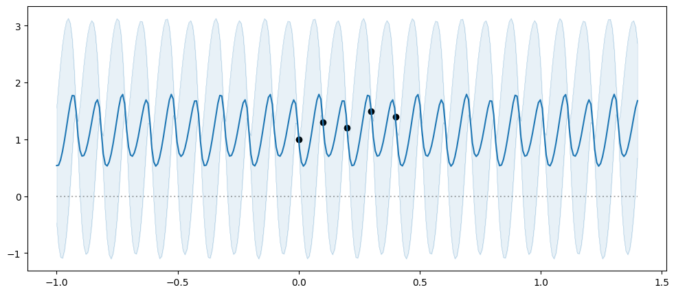
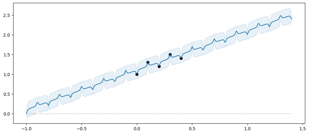
And combine them, we get a period around a line:

model = gpflow.models.GPR(
    (X, Y),
    kernel=gpflow.kernels.Periodic(gpflow.kernels.Matern32(), period=0.2),
    mean_function=gpflow.functions.Linear(),
    noise_variance=1e-3,
)
plot_model(model, min_x=-1.0, max_x=1.4)

Kernels versus mean functions

There is some overlap in what you can achieve with kernels and mean functions. If you have some external reason to expect your data to have a particular shape, we recommend you use that as a mean function. For example, you may be modelling a physical system where you have closed-form (physics) equations available that describes the system. However, if you do not have an external reason to pick a particular mean function we generally recommend you work on picking a good kernel, instead of setting a mean function. A good kernel will be better at “letting the data speak for itself”, whereas if you set a bad mean function, you can get misleading predictions.

Custom mean functions

It is easy enough to create a custom mean function. You must extend the gpflow.functions.MeanFunction class, which only requires you to implement a __call__ method. For example:

class SineMeanFunction(gpflow.functions.MeanFunction):
    @inherit_check_shapes
    def __call__(self, X: gpflow.base.TensorType) -> tf.Tensor:
        return tf.sin(X)


X = np.zeros((0, 1))
Y = np.zeros((0, 1))
model = gpflow.models.GPR(
    (X, Y),
    kernel=gpflow.kernels.Matern12(),
    mean_function=SineMeanFunction(),
)
plot_model(model, min_x=-15.0, max_x=15.0)

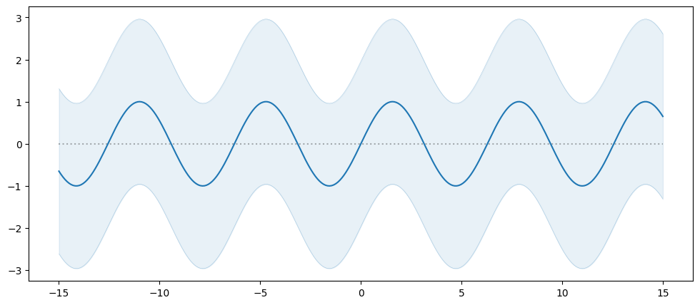
The above mean function does not have any trainable parameters. It is common for a mean function to have parameters that will be set during model training. To learn more about parameters see our section on Parameters and Their Optimisation.

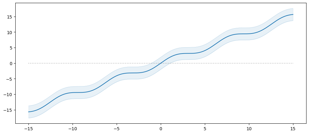
Composition

As with the kernels you can use the + and * operators to compose mean functions.

For example we can add a linear to our sine wave above:

model = gpflow.models.GPR(
    (X, Y),
    kernel=gpflow.kernels.Matern12(),
    mean_function=SineMeanFunction() + gpflow.functions.Linear(),
)
plot_model(model, min_x=-15.0, max_x=15.0)

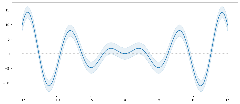
Or we can multiply the sine by a linear:

model = gpflow.models.GPR(
    (X, Y),
    kernel=gpflow.kernels.Matern12(),
    mean_function=SineMeanFunction() * gpflow.functions.Linear(),
)
plot_model(model, min_x=-15.0, max_x=15.0)