Monitoring

GPflow comes with a small framework for monitoring the training of your models. We will introduce this framework in this chapter.

Before we dive into monitoring however, let us have the usual imports, and let us create a small helper functions that creates a model we can monitor:

import matplotlib
import matplotlib.pyplot as plt
import numpy as np
import tensorflow as tf

import gpflow


X = np.array(
    [
        [0.865], [0.666], [0.804], [0.771], [0.147], [0.866], [0.007], [0.026],
        [0.171], [0.889], [0.243], [0.028],
    ]
)
Y = np.array(
    [
        [1.57], [3.48], [3.12], [3.91], [3.07], [1.35], [3.80], [3.82], [3.49],
        [1.30], [4.00], [3.82],
    ]
)


def get_model() -> gpflow.models.GPModel:
    return gpflow.models.GPR((X, Y), kernel=gpflow.kernels.SquaredExponential())

Components of monitoring

The most basic component of GPflow monitoring is the MonitorTask. Sub-classes of MonitorTask are responsible for actually doing the monitoring work.

MonitorTasks are grouped into MonitorTaskGroups, according to the frequency with which they are to be executed. So as not to impact training speed too much, MonitorTasks are generally not executed for every training iteration. Instead the MonitorTaskGroup is configured for how often the task should be executed.

Finally MonitorTaskGroups are grouped into one Monitor, which is the part that you pass to GPflow.

ExecuteCallback

The ExecuteCallback class implements MonitoringTask and allows you to wrap a simple Python function. Let us run the whole thing in an example:

model = get_model()


def my_callback() -> None:
    print("Hello, GPflow monitoring!")


execute_task = gpflow.monitor.ExecuteCallback(my_callback)
task_group = gpflow.monitor.MonitorTaskGroup(execute_task, period=3)
monitor = gpflow.monitor.Monitor(task_group)

opt = gpflow.optimizers.Scipy()
opt.minimize(
    model.training_loss, model.trainable_variables, step_callback=monitor
)

Hello, GPflow monitoring!
Hello, GPflow monitoring!
Hello, GPflow monitoring!
Hello, GPflow monitoring!
Hello, GPflow monitoring!
Hello, GPflow monitoring!

TensorBoard integration

The primary value of the GPFlow monitoring framework is however, its integration with TensorBoard. This gives you an easy way to export the progress of your training.

We will first demonstrate ModelToTensorBoard, which is an easy way to export your entire model:

model = get_model()
log_dir = "logs/model"

model_task = gpflow.monitor.ModelToTensorBoard(log_dir, model)
task_group = gpflow.monitor.MonitorTaskGroup(model_task, period=3)
monitor = gpflow.monitor.Monitor(task_group)

opt = gpflow.optimizers.Scipy()
opt.minimize(
    model.training_loss, model.trainable_variables, step_callback=monitor
)

Notice how we need to provide TensorBoard with a log directory. Generally TensorBoard reads and writes files from directories, and directories are the primary way you identify your runs. To view the logs you run something like:

tensorboard --logdir . --reload_multifile=true

The --reload_multifile=true is needed because the GPflow monitoring framework generally outputs multiple files.

You can use ScalarToTensorBoard to write arbitrary values to the logs. You need to provide a callback function that returns a scalar value; either a float, or a scalar tensor:

model = get_model()


def my_scalar() -> tf.Tensor:
    return model.training_loss()

Let us test our function first:

my_scalar()

<tf.Tensor: shape=(), dtype=float64, numpy=21.5778089200757>

And this is how we use it as a monitor:

log_dir = "logs/scalar"

scalar_task = gpflow.monitor.ScalarToTensorBoard(
    log_dir, my_scalar, "my_scalar_name"
)
task_group = gpflow.monitor.MonitorTaskGroup(scalar_task, period=3)
monitor = gpflow.monitor.Monitor(task_group)

opt = gpflow.optimizers.Scipy()
opt.minimize(
    model.training_loss, model.trainable_variables, step_callback=monitor
)

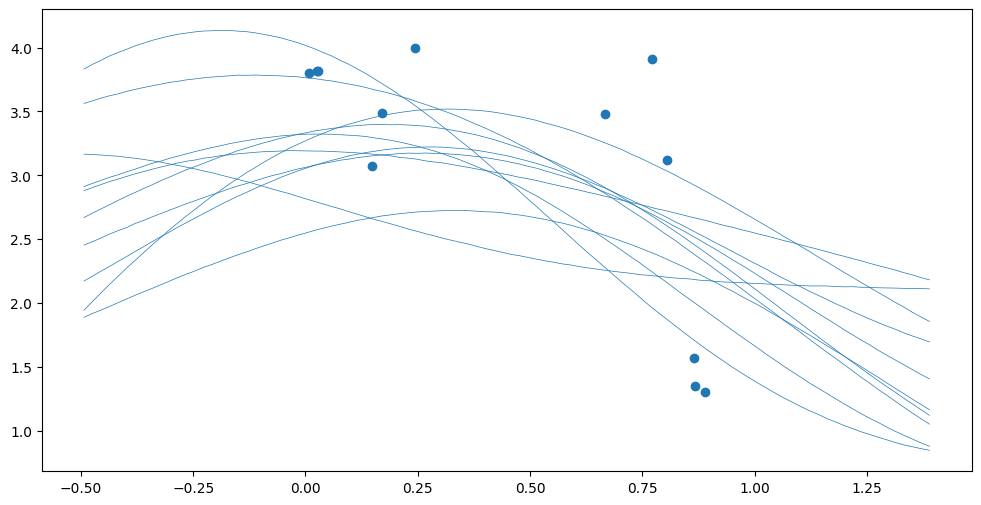
And you can use ImageToTensorBoard to write arbitrary images to the logs. In this case your callback function needs to take a matplotlib Figure and Axes, and plot your images to those:

model = get_model()


def my_image(
    figure: matplotlib.figure.Figure, ax: matplotlib.axes.Axes
) -> None:
    Xnew = np.linspace(X.min() - 0.5, X.max() + 0.5, 100)[:, None]
    Ypred = model.predict_f_samples(Xnew, full_cov=True, num_samples=10)
    ax.plot(Xnew.flatten(), np.squeeze(Ypred).T, "C0", lw=0.5)
    ax.scatter(X, Y)

Again, let us test our callback in isolation, before we use it:

fig, ax = plt.subplots()
my_image(fig, ax)

And this is how we use the callback:

log_dir = "logs/image"

image_task = gpflow.monitor.ImageToTensorBoard(
    log_dir, my_image, "my_image_name"
)
task_group = gpflow.monitor.MonitorTaskGroup(image_task, period=3)
monitor = gpflow.monitor.Monitor(task_group)

opt = gpflow.optimizers.Scipy()
opt.minimize(
    model.training_loss, model.trainable_variables, step_callback=monitor
)

Finally, let us demonstrate what it might look like if you use all these monitor tasks at the same time:

log_dir = "logs/combined"
model = get_model()


def my_scalar_2() -> tf.Tensor:
    return model.training_loss()


def my_image_2(
    figure: matplotlib.figure.Figure, ax: matplotlib.axes.Axes
) -> None:
    Xnew = np.linspace(X.min() - 0.5, X.max() + 0.5, 100)[:, None]
    Ypred = model.predict_f_samples(Xnew, full_cov=True, num_samples=10)
    ax.plot(Xnew.flatten(), np.squeeze(Ypred).T, "C0", lw=0.5)
    ax.scatter(X, Y)


model_task = gpflow.monitor.ModelToTensorBoard(log_dir, model)
scalar_task = gpflow.monitor.ScalarToTensorBoard(
    log_dir, my_scalar_2, "my_scalar_name"
)
image_task = gpflow.monitor.ImageToTensorBoard(
    log_dir, my_image_2, "my_image_name"
)

fast_task_group = gpflow.monitor.MonitorTaskGroup(
    [model_task, scalar_task], period=1
)
slow_task_group = gpflow.monitor.MonitorTaskGroup(image_task, period=3)

monitor = gpflow.monitor.Monitor(fast_task_group, slow_task_group)

opt = gpflow.optimizers.Scipy()
opt.minimize(
    model.training_loss, model.trainable_variables, step_callback=monitor
)

Here we needed to redefine my_scalar and my_image because we had hardcoded the model.

gpflow.optimizers.Scipy.minimize() runs an optimizer until convergence. Other optimizers, like tensorflow.keras.optimizers.Adam() need .minimize() to be called in a loop:

opt = tf.keras.optimizers.Adam()

@tf.function def optimization_step(): opt.minimize(model.training_loss, model.trainable_variables)

for i in range(10): optimization_step() monitor(i)