Saving and Loading Models

In this chapter we will talk about what we can do to save and restore GPflow models.

In the below we will demonstrate three different techniques: The two first are based on TensorFlow infrastructure: checkpoints and SavedModel, and the last one is how to use raw access to model parameters.

As usual we will start with some imports:

from typing import Callable, Tuple

import matplotlib.pyplot as plt
import numpy as np
import tensorflow as tf

import gpflow

Let us define some data to test with:

X = np.array(
    [
        [0.865], [0.666], [0.804], [0.771], [0.147], [0.866], [0.007], [0.026],
        [0.171], [0.889], [0.243], [0.028],
    ]
)
Y = np.array(
    [
        [1.57], [3.48], [3.12], [3.91], [3.07], [1.35], [3.80], [3.82], [3.49],
        [1.30], [4.00], [3.82],
    ]
)

And a helper function for plotting a model:

def plot_prediction(
    predict_y: Callable[[tf.Tensor], Tuple[tf.Tensor, tf.Tensor]]
) -> None:
    Xplot = np.linspace(0.0, 1.0, 200)[:, None]

    y_mean, y_var = predict_y(Xplot)
    y_lower = y_mean - 1.96 * np.sqrt(y_var)
    y_upper = y_mean + 1.96 * np.sqrt(y_var)

    _, ax = plt.subplots(nrows=1, ncols=1)
    ax.plot(X, Y, "kx", mew=2)
    (mean_line,) = ax.plot(Xplot, y_mean, "-")
    color = mean_line.get_color()
    ax.plot(Xplot, y_lower, lw=0.1, color=color)
    ax.plot(Xplot, y_upper, lw=0.1, color=color)
    ax.fill_between(
        Xplot[:, 0], y_lower[:, 0], y_upper[:, 0], color=color, alpha=0.1
    )

Checkpointing

Checkpoints are a mechanism built into TensorFlow, and they work out-of-the-box with GPflow.

With the help of tf.train.CheckpointManager and tf.train.Checkpoint, we can checkpoint the model throughout the training procedure. Let’s start with a simple example using checkpointing to save and load a tf.Variable:

initial_value = 1.2
a = tf.Variable(initial_value)

Create Checkpoint object:

log_dir = "checkpoints_0"
ckpt = tf.train.Checkpoint(a=a)
manager = tf.train.CheckpointManager(ckpt, log_dir, max_to_keep=3)

Save the variable a and change its value right after:

manager.save()
a.assign(0.33)

Now we can restore the old variable value:

print(f"Current value of variable a: {a.numpy():0.3f}")

ckpt.restore(manager.latest_checkpoint)

print(f"Value of variable a after restore: {a.numpy():0.3f}")

Current value of variable a: 0.330
Value of variable a after restore: 1.200

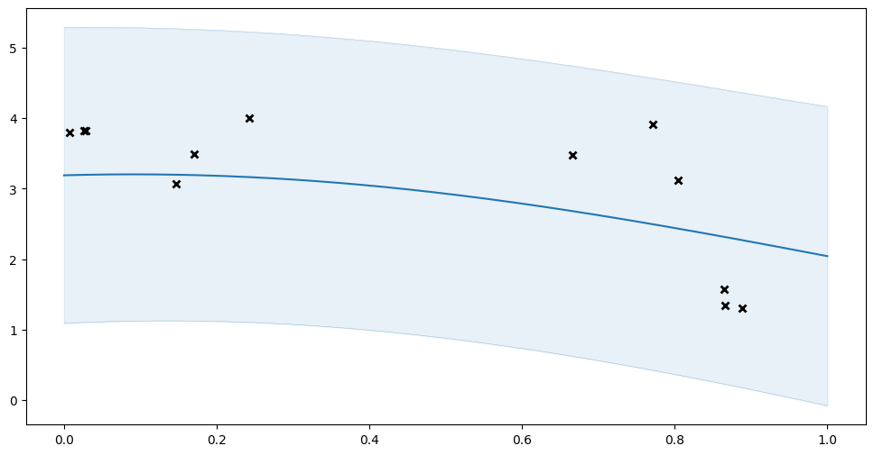
We can use this on entire GPflow models. First we define our model, checkpoint it, and show its fit before optimization:

model = gpflow.models.GPR((X, Y), kernel=gpflow.kernels.SquaredExponential())

log_dir = "checkpoints_1"
ckpt = tf.train.Checkpoint(model=model)
manager = tf.train.CheckpointManager(ckpt, log_dir, max_to_keep=3)
manager.save()

plot_prediction(model.predict_y)

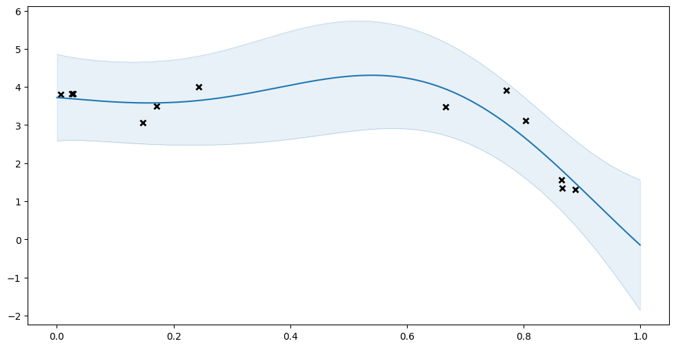
Now let us try optimizing the model:

opt = gpflow.optimizers.Scipy()
opt.minimize(model.training_loss, model.trainable_variables)
plot_prediction(model.predict_y)

Of course this is a better fit, but let us demonstrate that we can restore the un-optimised model:

ckpt.restore(manager.latest_checkpoint)
plot_prediction(model.predict_y)

Here is an example of how one might use the GPFlow monitoring framework to regularly checkpoint your model during training:

model = gpflow.models.GPR((X, Y), kernel=gpflow.kernels.SquaredExponential())

log_dir = "checkpoints_2"
ckpt = tf.train.Checkpoint(model=model)
manager = tf.train.CheckpointManager(ckpt, log_dir, max_to_keep=3)
manager.save()

checkpoint_task = gpflow.monitor.ExecuteCallback(manager.save)
task_group = gpflow.monitor.MonitorTaskGroup(checkpoint_task, period=3)
monitor = gpflow.monitor.Monitor(task_group)

opt = gpflow.optimizers.Scipy()
opt.minimize(
    model.training_loss, model.trainable_variables, step_callback=monitor
)

We can list the generated checkpoints to verify this worked. Remeber we set max_to_keep=3, so we expect to see three checkpoints:

manager.checkpoints

['checkpoints_2/ckpt-5', 'checkpoints_2/ckpt-6', 'checkpoints_2/ckpt-7']

TensorFlow saved_model

Another TensorFlow mechanism for model saving is saved_model.

saved_model only stores functions compiled with tf.function so we will have to compile anything we care about on our model. Notice that these “compiled” methods do not normally exist on our model, however in Python we can add any attributes we like to an object at any time:

hasattr(model, "compiled_predict_f")

False

model.compiled_predict_f = tf.function(
    lambda Xnew: model.predict_f(Xnew, full_cov=False),
    input_signature=[tf.TensorSpec(shape=[None, 1], dtype=tf.float64)],
)
model.compiled_predict_y = tf.function(
    lambda Xnew: model.predict_y(Xnew, full_cov=False),
    input_signature=[tf.TensorSpec(shape=[None, 1], dtype=tf.float64)],
)

save_dir = "saved_model_0"
tf.saved_model.save(model, save_dir)

We can load the module back as a new instance and compare the prediction results:

loaded_model = tf.saved_model.load(save_dir)

plot_prediction(model.predict_y)
plot_prediction(loaded_model.compiled_predict_y)

Again notice that the regular methods, that have not been compiled, do not exist on our restored object:

hasattr(loaded_model, "predict_f")

False

Copying (hyper)parameter values between models

GPFlow comes with the functions gpflow.utilities.parameter_dict and gpflow.utilities.multiple_assign that allows you to get and set all parameters of a model. This makes it easy to copy all parameters from one model to another.

We can get the parameters of our model with parameter_dict:

model_0 = gpflow.models.GPR((X, Y), kernel=gpflow.kernels.SquaredExponential())

opt = gpflow.optimizers.Scipy()
opt.minimize(model_0.training_loss, model_0.trainable_variables)

gpflow.utilities.parameter_dict(model_0)

{'.kernel.variance': <Parameter: name=softplus, dtype=float64, shape=[], fn="softplus", numpy=11.646614675731874>,
 '.kernel.lengthscales': <Parameter: name=softplus, dtype=float64, shape=[], fn="softplus", numpy=0.3733319087937649>,
 '.likelihood.variance': <Parameter: name=chain_of_shift_of_softplus, dtype=float64, shape=[], fn="chain_of_shift_of_softplus", numpy=0.24001197623266737>}

And we can use multiple_assign to assign these parameters to a new model:

model_1 = gpflow.models.GPR((X, Y), kernel=gpflow.kernels.SquaredExponential())
params_0 = gpflow.utilities.parameter_dict(model_0)
gpflow.utilities.multiple_assign(model_1, params_0)

plot_prediction(model_0.predict_y)
plot_prediction(model_1.predict_y)

Which method to use

We have presented three different ways to save and load a model:

• Checkpointing.

• saved_model.

• parameter_dict + multiple_assign.

So, which one should you use?

Checkpointing should mostly be used for restarting / resuming training. Notice that checkpointing requires you to create a new model with exactly the same set-up as the old model, before you can restore your parameters. This means you must have access to the same Python code. Checkpointing also requires you to read / write files to disk.

saved_model is good when you want to create and train a model on one computer, but use it on another computer. With saved_model you do not need to create a model first, and then update parameters. Instead you are given a functioning model directly. This means you do not need to have access to the same Python code that created the model, on the computer that loads the model. The disadvantage is that a lot of the model will be lost in the process, so this is not useful if you want to make changes to your model later.

The parameter_dict and multiple_assign method is recommended if you want to make changes to your model after loading it. Again the machine loading the model will need to have access to code that created the model, to be able to instantiate a new model with the same set-up. Notice that this approach does not actually store the model on disk, but only makes an in-memory copy of the parameters. This is an advantage if you want to create multiple copies of a model in memory, but it means you will have to write your own code to read / write the parameter dictionaries if you want to store them to disk.