Parameters and Their Optimisation#
In this chapter we will talk about what happens when you train your model, and what you can do if the optimisation process fails to find a good fit.
As usual we start with some imports:
[1]:
from typing import Optional

import matplotlib.pyplot as plt
import numpy as np
import pandas as pd
import tensorflow as tf
import tensorflow_probability as tfp
from check_shapes import check_shapes
from matplotlib.axes import Axes

import gpflow
The Module and Parameter classes#
The two fundamental classes of GPflow are: * gpflow.Parameter. Parameters are leaf nodes holding numerical values, that can be tuned / trained to make the model fit the data. * gpflow.Module. Modules recursively composes other modules and parameters to create models. All the GPflow models, kernels, mean functions, etc. are modules.
As an example, let’s build a simple linear model:
[2]:
class LinearModel(gpflow.Module):
    @check_shapes(
        "slope: [n_inputs, n_outputs]",
        "bias: [n_outputs]",
    )
    def __init__(
        self, slope: gpflow.base.TensorData, bias: gpflow.base.TensorData
    ) -> None:
        super().__init__()
        self.slope = gpflow.Parameter(slope)
        self.bias = gpflow.Parameter(bias)

    @check_shapes(
        "X: [n_rows, n_inputs]",
        "return: [n_rows, n_outputs]",
    )
    def predict(self, X: gpflow.base.TensorData) -> tf.Tensor:
        return X @ self.slope + self.bias[:, None]
Notice that in __init__ we directly pass data to the parameters. The Parameter class takes many arguments (which we will discuss below), but it is reasonably intelligent as in: We can pass it “raw” numerical values with a Python list, a NumPy array, or a TensorFlow tensor; or we can pass it another Parameter and it will take values from that. Being able to pass a Parameter to __init__ gives us a convenient way to configure the parameter in detail.
Inspecting parameters#
Let’s first create an instance of our LinearModel:
[3]:
model = LinearModel([[1.0], [2.0]], [0.5])
We can use the GPflow utility functions print_summary to see a summary of anything extending the GPflow Module:
[4]:
gpflow.utilities.print_summary(model)
╒═══════════════════╤═══════════╤═════════════╤═════════╤═════════════╤═════════╤═════════╤═════════╕
│ name              │ class     │ transform   │ prior   │ trainable   │ shape   │ dtype   │ value   │
╞═══════════════════╪═══════════╪═════════════╪═════════╪═════════════╪═════════╪═════════╪═════════╡
│ LinearModel.slope │ Parameter │ Identity    │         │ True        │ (2, 1)  │ float64 │ [[1.]   │
│                   │           │             │         │             │         │         │  [2.]]  │
├───────────────────┼───────────┼─────────────┼─────────┼─────────────┼─────────┼─────────┼─────────┤
│ LinearModel.bias  │ Parameter │ Identity    │         │ True        │ (1,)    │ float64 │ [0.5]   │
╘═══════════════════╧═══════════╧═════════════╧═════════╧═════════════╧═════════╧═════════╧═════════╛
Looking at the output of print_summary. The name and class columns should be obvious if you’re familiar with Python. We’re also assuming that you’re comfortable with NumPy and TensorFlow so the last three columns shape, dtype, and value should also be obvious. The three middle columns transform, prior and trainable will be explained below.
We generally recommend printing your parameter values after model traning, to sanity check them, and to develop a feel for what parameters are a good fit for your data.
print_summary has nice integration with Jupyter Notebooks:
[5]:
gpflow.utilities.print_summary(model, "notebook")
| name | class | transform | prior | trainable | shape | dtype | value |
|---|---|---|---|---|---|---|---|
| LinearModel.slope | Parameter | Identity | True | (2, 1) | float64 | [[1.] [2.]] | |
| LinearModel.bias | Parameter | Identity | True | (1,) | float64 | [0.5] |
And we can configure GPflow to use the notebook format by default:
[6]:
gpflow.config.set_default_summary_fmt("notebook")
gpflow.utilities.print_summary(model)
| name | class | transform | prior | trainable | shape | dtype | value |
|---|---|---|---|---|---|---|---|
| LinearModel.slope | Parameter | Identity | True | (2, 1) | float64 | [[1.] [2.]] | |
| LinearModel.bias | Parameter | Identity | True | (1,) | float64 | [0.5] |
Alternatively Modules know how to print themselves nicely in a notebook:
[7]:
model
[7]:
| name | class | transform | prior | trainable | shape | dtype | value |
|---|---|---|---|---|---|---|---|
| LinearModel.slope | Parameter | Identity | True | (2, 1) | float64 | [[1.] [2.]] | |
| LinearModel.bias | Parameter | Identity | True | (1,) | float64 | [0.5] |
Finally, a Module has two properties that allows easy access to its leaf parameters:
[8]:
model.parameters
[8]:
(<Parameter: name=identity, dtype=float64, shape=[1], fn="identity", numpy=array([0.5])>,
 <Parameter: name=identity, dtype=float64, shape=[2, 1], fn="identity", numpy=
 array([[1.],
        [2.]])>)
[9]:
model.trainable_parameters
[9]:
(<Parameter: name=identity, dtype=float64, shape=[1], fn="identity", numpy=array([0.5])>,
 <Parameter: name=identity, dtype=float64, shape=[2, 1], fn="identity", numpy=
 array([[1.],
        [2.]])>)
The difference between trainable and non-trainable parameters will be explained further below. For now you may notice that both our parameters are marked “trainable” in the print_summary output, and both of them are returned by .trainable_parameters.
Generally you should use print_summary to manually inspect your models, and .parameters and .trainable_parameters if you need programmatic access.
Setting parameters#
Parameters have a .assign method you can use to set them:
[10]:
model.bias.assign([5.0])
gpflow.utilities.print_summary(model)
| name | class | transform | prior | trainable | shape | dtype | value |
|---|---|---|---|---|---|---|---|
| LinearModel.slope | Parameter | Identity | True | (2, 1) | float64 | [[1.] [2.]] | |
| LinearModel.bias | Parameter | Identity | True | (1,) | float64 | [5.] |
Optimisation#
The objective of optimisation is to change the parameters so that your model fits the data. Generally an optimiser takes a “loss” function and a list of parameters, it then changes the parameters to minimise the loss function.
Let’s us try to optimise our LinearModel.
First we need some data. This data is computed manually, given \(y_i = 2x_{i0} + 3x_{i1} + 1\).
[11]:
X_train = np.array([[0, 0], [0, 2], [1, 0], [3, 2]])
Y_train = np.array([[1], [7], [3], [13]])
Next we need our loss function. A common choice is the mean squared error:
[12]:
def loss() -> tf.Tensor:
    Y_predicted = model.predict(X_train)
    squared_error = (Y_predicted - Y_train) ** 2
    return tf.reduce_mean(squared_error)
Be aware that GPflow’s own models all come with a loss-function predefined — use model.training_loss.
Now we can plug this into the default GPflow optimiser:
[13]:
opt = gpflow.optimizers.Scipy()
opt.minimize(loss, model.trainable_variables)
gpflow.utilities.print_summary(model)
| name | class | transform | prior | trainable | shape | dtype | value |
|---|---|---|---|---|---|---|---|
| LinearModel.slope | Parameter | Identity | True | (2, 1) | float64 | [[2.] [3.]] | |
| LinearModel.bias | Parameter | Identity | True | (1,) | float64 | [1.] |
Notice how the optimiser recovered the slope of \((2, 3)\) and bias of \(1\) from the equation we used to generate the data: \(y_i = 2x_{i0} + 3x_{i1} + 1\).
The default GPflow optimiser uses a gradient descent method called BFGS. For this algoritm to work well you need:
A deterministic loss function. Notice this rules out mini-batching, because the random batches inject randomness into the loss function.
Not too many parameters. You will probably be fine up to a couple of thousand parameters.
What to do if you model fails to fit#
In our above example the optimiser perfectly recovered the parameters of the process that generated our data. However, it was a very easy problem we were solving. As you start working with more complicated data sets you may find that the optimiser fails to find a good fit for you model. In this section we will discuss what you can do to help the optimiser a bit.
Dataset: \(CO_2\) levels#
As an example we will use a dataset of atmospheric \(CO_2\) levels, as measured at the Mauna Loa observatory in Hawaii:
[14]:
co2_data = pd.read_csv(
    "https://gml.noaa.gov/webdata/ccgg/trends/co2/co2_mm_mlo.csv", comment="#"
)
Xco2 = co2_data["decimal date"].values[:, None]
Yco2 = co2_data["average"].values[:, None]
And we will define some helper functions to train and plot a model with the data:
[15]:
def plot_co2_model_prediction(
    ax: Axes, model: gpflow.models.GPModel, start: float, stop: float
) -> None:
    Xplot = np.linspace(start, stop, 200)[:, None]
    idx_plot = (start < Xco2) & (Xco2 < stop)

    y_mean, y_var = model.predict_y(Xplot, full_cov=False)
    y_lower = y_mean - 1.96 * np.sqrt(y_var)
    y_upper = y_mean + 1.96 * np.sqrt(y_var)

    ax.plot(Xco2[idx_plot], Yco2[idx_plot], "kx", mew=2)
    (mean_line,) = ax.plot(Xplot, y_mean, "-")
    color = mean_line.get_color()
    ax.plot(Xplot, y_lower, lw=0.1, color=color)
    ax.plot(Xplot, y_upper, lw=0.1, color=color)
    ax.fill_between(
        Xplot[:, 0], y_lower[:, 0], y_upper[:, 0], color=color, alpha=0.1
    )


opt_options = dict(maxiter=100)


def plot_co2_kernel(
    kernel: gpflow.kernels.Kernel,
    *,
    optimize: bool = False,
) -> None:
    model = gpflow.models.GPR(
        (Xco2, Yco2),
        kernel=kernel,
    )
    if optimize:
        opt = gpflow.optimizers.Scipy()
        opt.minimize(
            model.training_loss, model.trainable_variables, options=opt_options
        )
    gpflow.utilities.print_summary(model, "notebook")

    _, (ax1, ax2) = plt.subplots(nrows=1, ncols=2)
    plot_co2_model_prediction(ax1, model, 1950, 2050)
    plot_co2_model_prediction(ax2, model, 2015, 2030)
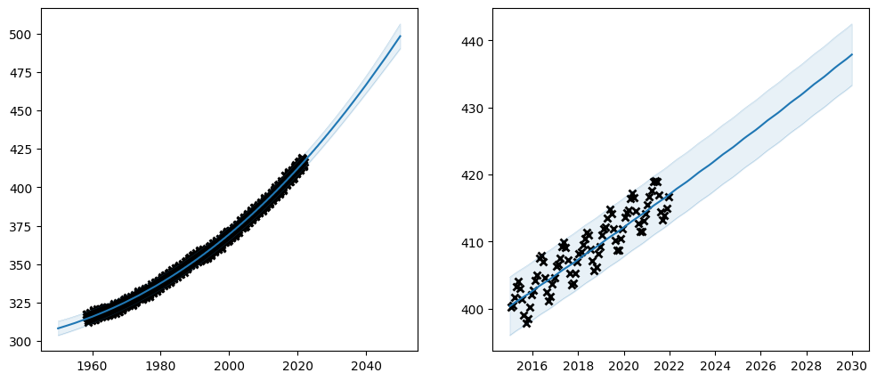
Let us start by trying to fit our favourite kernel: the squared exponential:
[16]:
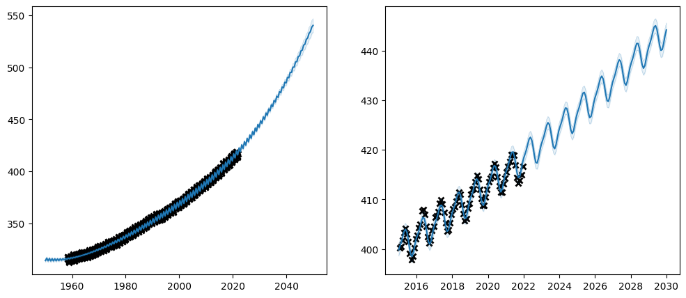
plot_co2_kernel(gpflow.kernels.SquaredExponential(), optimize=True)
| name | class | transform | prior | trainable | shape | dtype | value |
|---|---|---|---|---|---|---|---|
| GPR.kernel.variance | Parameter | Softplus | True | () | float64 | 91524.8 | |
| GPR.kernel.lengthscales | Parameter | Softplus | True | () | float64 | 47.7904 | |
| GPR.likelihood.variance | Parameter | Softplus + Shift | True | () | float64 | 4.72387 |

We are off to a good start. From the left plot it is clear that the kernel has captured the long-term trend of the data. However, on the zoomed-in plot on the right it is also clear that the data has some kind of yearly cycle that our model has failed to capture.
Let us try adding a periodic kernel to capture the yearly cycle:
[17]:
plot_co2_kernel(
    gpflow.kernels.SquaredExponential()
    + gpflow.kernels.Periodic(gpflow.kernels.SquaredExponential()),
    optimize=True,
)
| name | class | transform | prior | trainable | shape | dtype | value |
|---|---|---|---|---|---|---|---|
| GPR.kernel.kernels[0].variance | Parameter | Softplus | True | () | float64 | 25719.6 | |
| GPR.kernel.kernels[0].lengthscales | Parameter | Softplus | True | () | float64 | 42.3687 | |
| GPR.kernel.kernels[1].base_kernel.variance | Parameter | Softplus | True | () | float64 | 34714.7 | |
| GPR.kernel.kernels[1].base_kernel.lengthscales | Parameter | Softplus | True | () | float64 | 1599.5 | |
| GPR.kernel.kernels[1].period | Parameter | Softplus | True | () | float64 | 100.539 | |
| GPR.likelihood.variance | Parameter | Softplus + Shift | True | () | float64 | 4.72205 |
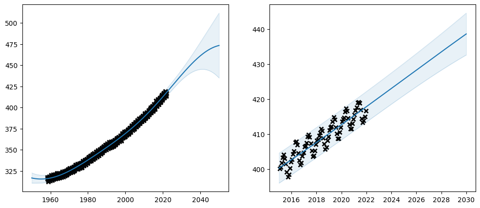
Huh. What happened? The optimiser has failed to find a good fit. With the extended model the loss function has become too complicated for the optimiser.
Below we will look at what we can do to help the optimiser.
Setting the initial value#
The simplest thing you can do to help the optimiser is to set your parameters to good inital values.
When we just fit a single
SquaredExponentialto the data we got great values for the long term trend. Let us reuse those parameters.We know that we intend the periodic kernel to capture a yearly cycle. The units on the X-axis are years, so the period should be 1.
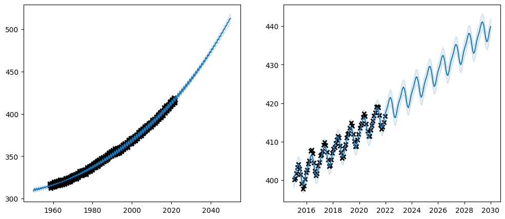
Let us try simply setting the parameters of our long-term-trend kernel to approximately those learned when it was trained individually, and the period to 1:
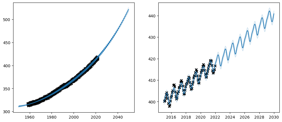
[18]:
plot_co2_kernel(
    gpflow.kernels.SquaredExponential(variance=280_000, lengthscales=140.0)
    + gpflow.kernels.Periodic(gpflow.kernels.SquaredExponential(), period=1.0),
    optimize=True,
)
| name | class | transform | prior | trainable | shape | dtype | value |
|---|---|---|---|---|---|---|---|
| GPR.kernel.kernels[0].variance | Parameter | Softplus | True | () | float64 | 280000 | |
| GPR.kernel.kernels[0].lengthscales | Parameter | Softplus | True | () | float64 | 15.6477 | |
| GPR.kernel.kernels[1].base_kernel.variance | Parameter | Softplus | True | () | float64 | 186.998 | |
| GPR.kernel.kernels[1].base_kernel.lengthscales | Parameter | Softplus | True | () | float64 | 1.8148 | |
| GPR.kernel.kernels[1].period | Parameter | Softplus | True | () | float64 | 0.999617 | |
| GPR.likelihood.variance | Parameter | Softplus + Shift | True | () | float64 | 0.208541 |
Priors#
It it always a good idea to try to set reasonable initial values on your parameters. However, it is not always enough. An initial value is just a starting point, and the optimiser may in principle choose any value whatsever for the final value. Another, possibly more principled, approach to guiding the optimiser is to set a “prior” on your parameters. A prior is a probability distribution that represents your belief of what the parameter should be, before the optimiser takes the data into account. We use the TensorFlow Probability Distribution class to represent priors.
There are two ways to apply a prior to your parameters. First, you can create the parameter with the prior:
[19]:
p = gpflow.Parameter(1.0, prior=tfp.distributions.Normal(loc=1.0, scale=10.0))
Or you can create the parameter first, and then set the prior:
[20]:
p = gpflow.Parameter(1.0)
p.prior = tfp.distributions.Normal(loc=1.0, scale=10.0)
Let us try using priors on our \(CO_2\) model:
[21]:
long_term_kernel = gpflow.kernels.SquaredExponential()
long_term_kernel.variance.prior = tfp.distributions.LogNormal(
tf.math.log(gpflow.utilities.to_default_float(280_000.0)), 1.0
)
long_term_kernel.lengthscales.prior = tfp.distributions.LogNormal(
tf.math.log(gpflow.utilities.to_default_float(140.0)), 0.05
)
periodic_kernel = gpflow.kernels.Periodic(gpflow.kernels.SquaredExponential())
periodic_kernel.period.prior = tfp.distributions.LogNormal(
tf.math.log(gpflow.utilities.to_default_float(1.0)), 0.1
)
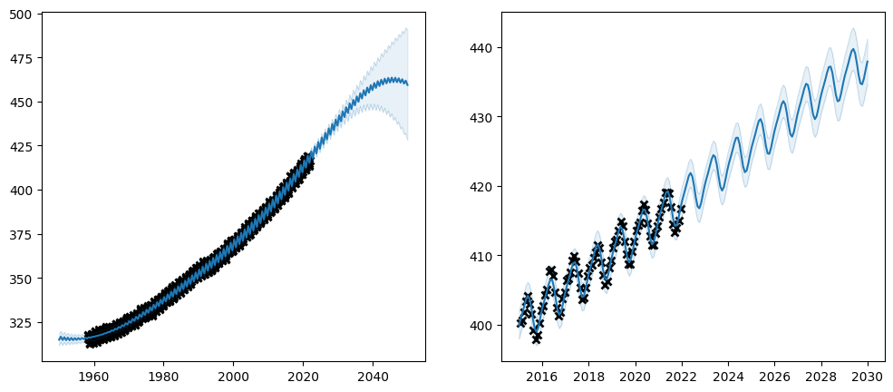
plot_co2_kernel(long_term_kernel + periodic_kernel, optimize=True)
| name | class | transform | prior | trainable | shape | dtype | value |
|---|---|---|---|---|---|---|---|
| GPR.kernel.kernels[0].variance | Parameter | Softplus | LogNormal | True | () | float64 | 170883 |
| GPR.kernel.kernels[0].lengthscales | Parameter | Softplus | LogNormal | True | () | float64 | 139.393 |
| GPR.kernel.kernels[1].base_kernel.variance | Parameter | Softplus | True | () | float64 | 154051 | |
| GPR.kernel.kernels[1].base_kernel.lengthscales | Parameter | Softplus | True | () | float64 | 15301.9 | |
| GPR.kernel.kernels[1].period | Parameter | Softplus | LogNormal | True | () | float64 | 0.999549 |
| GPR.likelihood.variance | Parameter | Softplus + Shift | True | () | float64 | 4.87244 |
Notice that many parameters have constraints on what values are valid. In this case all of variance, lengthscales and period should be non-negative. That is why we chose the LogNormal distribution for our prior - it only allows positive values.
Also notice in our table of parameters, that the prior column now shows LogNormal for the parameters we set the prior on.
Transforms#
As mentioned above, some parameters have constraints on what values are valid. GPflow uses “transforms” to enforce this. The parameter stores a raw value that can be anything. When you read the parameter that value is sent through a function, the “transform”, that maps the entire real line to the set of valid values. We use the TensorFlow Probability Bijector class for the transform.
You can only set the transform of a parameter when you create it. For example:
[22]:
p = gpflow.Parameter(1.0, transform=tfp.bijectors.Exp())
In this example we used the exponential function as a transform. Since the exponential functions maps the entire real line to positive values this transform will ensure that the parameter always take positive values.
We can access the untransformed value of the parameter:
[23]:
p.unconstrained_variable
[23]:
<tf.Variable 'exp:0' shape=() dtype=float64, numpy=0.0>
[24]:
p.unconstrained_variable.assign(-3)
[24]:
<tf.Variable 'UnreadVariable' shape=() dtype=float64, numpy=-3.0>
When we read the parameter we will read the transformed value, which is positive, even though we just set the untransformed value to a negative number:
[25]:
p
[25]:
<Parameter: name=exp, dtype=float64, shape=[], fn="exp", numpy=0.049787068367863944>
Let us try and use transforms on our \(CO_2\) problem:
[26]:
long_term_kernel = gpflow.kernels.SquaredExponential()
long_term_kernel.variance = gpflow.Parameter(
    280_000,
    transform=tfp.bijectors.SoftClip(
        gpflow.utilities.to_default_float(200_000),
        gpflow.utilities.to_default_float(400_000),
    ),
)
long_term_kernel.lengthscales = gpflow.Parameter(
    140,
    transform=tfp.bijectors.SoftClip(
        gpflow.utilities.to_default_float(100),
        gpflow.utilities.to_default_float(200),
    ),
)

periodic_kernel = gpflow.kernels.Periodic(gpflow.kernels.SquaredExponential())
periodic_kernel.period = gpflow.Parameter(
    1.0,
    transform=tfp.bijectors.SoftClip(
        gpflow.utilities.to_default_float(0.9),
        gpflow.utilities.to_default_float(1.1),
    ),
)

plot_co2_kernel(long_term_kernel + periodic_kernel, optimize=True)
| name | class | transform | prior | trainable | shape | dtype | value |
|---|---|---|---|---|---|---|---|
| GPR.kernel.kernels[0].variance | Parameter | SoftClip | True | () | float64 | 280000 | |
| GPR.kernel.kernels[0].lengthscales | Parameter | SoftClip | True | () | float64 | 100.002 | |
| GPR.kernel.kernels[1].base_kernel.variance | Parameter | Softplus | True | () | float64 | 62.6799 | |
| GPR.kernel.kernels[1].base_kernel.lengthscales | Parameter | Softplus | True | () | float64 | 1.44431 | |
| GPR.kernel.kernels[1].period | Parameter | SoftClip | True | () | float64 | 0.99962 | |
| GPR.likelihood.variance | Parameter | Softplus + Shift | True | () | float64 | 0.375282 |
Again, be aware that many parameters have constraints on what kind of values they logically can take, and if you replace the transform of a parameter you must make sure that the transform only allows values that are logically valid in the context in which they are used.
Also, notice how the values of the transform column in our parameter summary has updated to reflect our new transforms.
Trainable parameters#
In this section we have been going from setting initial parameter values, which are a very soft hint, over priors to transforms, which are more forceful ways of constraining the training process. The last step is to completely prevent the optimiser from changing a value. We can do that by setting the parameter to not be “trainable”.
You can set the trainability of a parameter either when you create it, or using the gpflow.set_trainable function:
[27]:
p = gpflow.Parameter(1.0, trainable=False)
[28]:
p = gpflow.Parameter(1.0)
gpflow.set_trainable(p, False)
The gpflow.set_trainable function can both be applied directly to parameters, or to modules, in which case all parameters held in the module are affected.
Let us try setting the trainability on our \(CO_2\) model:
[29]:
long_term_kernel = gpflow.kernels.SquaredExponential(
    variance=280_000, lengthscales=140
)
gpflow.set_trainable(long_term_kernel, False)

periodic_kernel = gpflow.kernels.Periodic(
    gpflow.kernels.SquaredExponential(), period=1
)
gpflow.set_trainable(periodic_kernel.period, False)

plot_co2_kernel(long_term_kernel + periodic_kernel, optimize=True)
| name | class | transform | prior | trainable | shape | dtype | value |
|---|---|---|---|---|---|---|---|
| GPR.kernel.kernels[0].variance | Parameter | Softplus | False | () | float64 | 280000 | |
| GPR.kernel.kernels[0].lengthscales | Parameter | Softplus | False | () | float64 | 140 | |
| GPR.kernel.kernels[1].base_kernel.variance | Parameter | Softplus | True | () | float64 | 44.6271 | |
| GPR.kernel.kernels[1].base_kernel.lengthscales | Parameter | Softplus | True | () | float64 | 1.32482 | |
| GPR.kernel.kernels[1].period | Parameter | Softplus | False | () | float64 | 1 | |
| GPR.likelihood.variance | Parameter | Softplus + Shift | True | () | float64 | 0.466 |
Notice how the trainable column of the parameter table reflects the whether the parameters are trainable. Also notice how the final value of the un-trainable parameters have exactly the value we initialised them to. Setting a parameter untrainable is a heavy-handed tool, and we generally recommend using one of the softer methods demonstrated above.
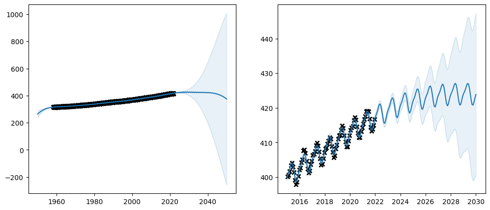
Advanced training#
Multi-stage training#
Remember how we first trained a model with only a SquaredExponential kernel, and in the above subsections we have been using parameters learned from that experiment for the initial values in a more complicated kernel?
What if you do not have access to the data when you write your code, and you can not “copy and paste” from a previous experiment? Well, it is possible to run optimisation multiple times, so we can start by running optimisation on a smaller set of parameters, which is a simpler problem to optimise; and then optimise all the parameters in a second run.
[30]:
# First we only use, and optimise, the long_term_kernel:
long_term_kernel = gpflow.kernels.SquaredExponential()

model = gpflow.models.GPR((Xco2, Yco2), kernel=long_term_kernel)
opt = gpflow.optimizers.Scipy()
opt.minimize(
    model.training_loss, model.trainable_variables, options=opt_options
)

# And then we use, and optimise, the full kernel:
periodic_kernel = gpflow.kernels.Periodic(gpflow.kernels.SquaredExponential())

kernel = long_term_kernel + periodic_kernel
model = gpflow.models.GPR((Xco2, Yco2), kernel=long_term_kernel)
opt = gpflow.optimizers.Scipy()
opt.minimize(
    model.training_loss, model.trainable_variables, options=opt_options
)

plot_co2_kernel(kernel, optimize=False)
| name | class | transform | prior | trainable | shape | dtype | value |
|---|---|---|---|---|---|---|---|
| GPR.kernel.kernels[0].variance | Parameter | Softplus | True | () | float64 | 91524.8 | |
| GPR.kernel.kernels[0].lengthscales | Parameter | Softplus | True | () | float64 | 47.7854 | |
| GPR.kernel.kernels[1].base_kernel.variance | Parameter | Softplus | True | () | float64 | 1 | |
| GPR.kernel.kernels[1].base_kernel.lengthscales | Parameter | Softplus | True | () | float64 | 1 | |
| GPR.kernel.kernels[1].period | Parameter | Softplus | True | () | float64 | 1 | |
| GPR.likelihood.variance | Parameter | Softplus + Shift | True | () | float64 | 1 |
The Keras optimisers#
So far we have been using the optimiser from GPflow. However, GPflow is built on TensorFlow variables and automatic differentiation, and you can use any other optimiser built on those as well. Here is an example of using a Keras optimiser with a TensorFlow model:
[31]:
model = gpflow.models.GPR(
    (Xco2, Yco2),
    kernel=gpflow.kernels.SquaredExponential(
        variance=280_000, lengthscales=140.0
    )
    + gpflow.kernels.Periodic(gpflow.kernels.SquaredExponential(), period=1.0),
)

opt = tf.keras.optimizers.Adam()


@tf.function
def step() -> tf.Tensor:
    opt.minimize(model.training_loss, model.trainable_variables)


maxiter = 2_000
for i in range(maxiter):
    step()
    if i % 100 == 0:
        print(i, model.training_loss().numpy())

kernel = model.kernel
plot_co2_kernel(kernel, optimize=False)
0 991.4059442406201
100 971.7466509519725
200 955.6740668954221
300 941.5794081194115
400 929.2696110890437
500 918.6005611346995
600 909.460132448887
700 901.7489538323437
800 895.3681923208954
900 890.195266609257
1000 886.1023264301939
1100 882.9433497245323
1200 880.5509597948467
1300 878.770548638013
1400 877.452415144139
1500 876.4629388068214
1600 875.7293761418225
1700 875.0827608578506
1800 874.5576038789667
1900 874.0889011747782
| name | class | transform | prior | trainable | shape | dtype | value |
|---|---|---|---|---|---|---|---|
| GPR.kernel.kernels[0].variance | Parameter | Softplus | True | () | float64 | 280002 | |
| GPR.kernel.kernels[0].lengthscales | Parameter | Softplus | True | () | float64 | 137.551 | |
| GPR.kernel.kernels[1].base_kernel.variance | Parameter | Softplus | True | () | float64 | 1.80474 | |
| GPR.kernel.kernels[1].base_kernel.lengthscales | Parameter | Softplus | True | () | float64 | 0.552585 | |
| GPR.kernel.kernels[1].period | Parameter | Softplus | True | () | float64 | 0.99962 | |
| GPR.likelihood.variance | Parameter | Softplus + Shift | True | () | float64 | 1 |