Classification, other data distributions, VGP and SVGP

In this chapter we will talk about what you can do if your data is not normally distributed.

As usual we will start with our imports:

from typing import Sequence

import matplotlib.pyplot as plt
import numpy as np

import gpflow

The Variational Gaussion Process

Remember how we assume that our data is generated by:

\begin{equation} Y_i = f(X_i) + \varepsilon_i \,, \quad \varepsilon_i \sim \mathcal{N}(0, \sigma^2). \end{equation}

In this chapter we will no longer assume this — instead we will allow any stochastic function of \(f\).

We will be using the Variational Gaussian Process (VGP) model in this chapter. The VGP uses a Likelihood object to define the connection between \(f\) and \(Y\). The models we have seen so far, the GPR and SGPR, requires the likelihood to be gaussian, but the VGP allows us to configure the likelihood.

Non-gaussian regression

Let us first define a helper function, for plotting a model:

def plot_model(model: gpflow.models.GPModel) -> None:
    X, Y = model.data
    opt = gpflow.optimizers.Scipy()
    opt.minimize(model.training_loss, model.trainable_variables)
    gpflow.utilities.print_summary(model, "notebook")

    Xplot = np.linspace(0.0, 1.0, 200)[:, None]

    y_mean, y_var = model.predict_y(Xplot, full_cov=False)
    y_lower = y_mean - 1.96 * np.sqrt(y_var)
    y_upper = y_mean + 1.96 * np.sqrt(y_var)

    _, ax = plt.subplots(nrows=1, ncols=1)
    ax.plot(X, Y, "kx", mew=2)
    (mean_line,) = ax.plot(Xplot, y_mean, "-")
    color = mean_line.get_color()
    ax.plot(Xplot, y_lower, lw=0.1, color=color)
    ax.plot(Xplot, y_upper, lw=0.1, color=color)
    ax.fill_between(
        Xplot[:, 0], y_lower[:, 0], y_upper[:, 0], color=color, alpha=0.1
    )

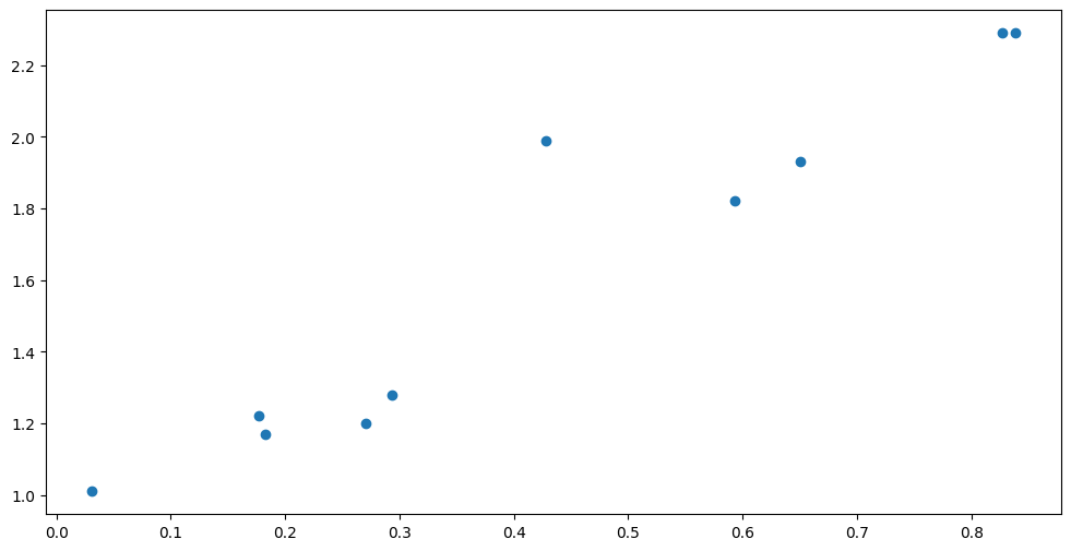
Below we have a small dataset with an outlier. The default Gaussian likelihood has very light tails, and will struggle with the outlier:

X = np.array(
    [
        [0.177], [0.183], [0.428], [0.838], [0.827], [0.293], [0.270], [0.593],
        [0.031], [0.650],
    ]
)
Y = np.array(
    [
        [1.22], [1.17], [1.99], [2.29], [2.29], [1.28], [1.20], [1.82], [1.01],
        [1.93],
    ]
)

plt.scatter(X, Y)

Let us try fitting the usual GPR to this data:

model: gpflow.models.GPModel = gpflow.models.GPR(
    (X, Y), kernel=gpflow.kernels.SquaredExponential()
)
plot_model(model)

name	class	transform	prior	trainable	shape	dtype	value
GPR.kernel.variance	Parameter	Softplus		True	()	float64	4.39101
GPR.kernel.lengthscales	Parameter	Softplus		True	()	float64	1.60446
GPR.likelihood.variance	Parameter	Softplus + Shift		True	()	float64	0.0243669

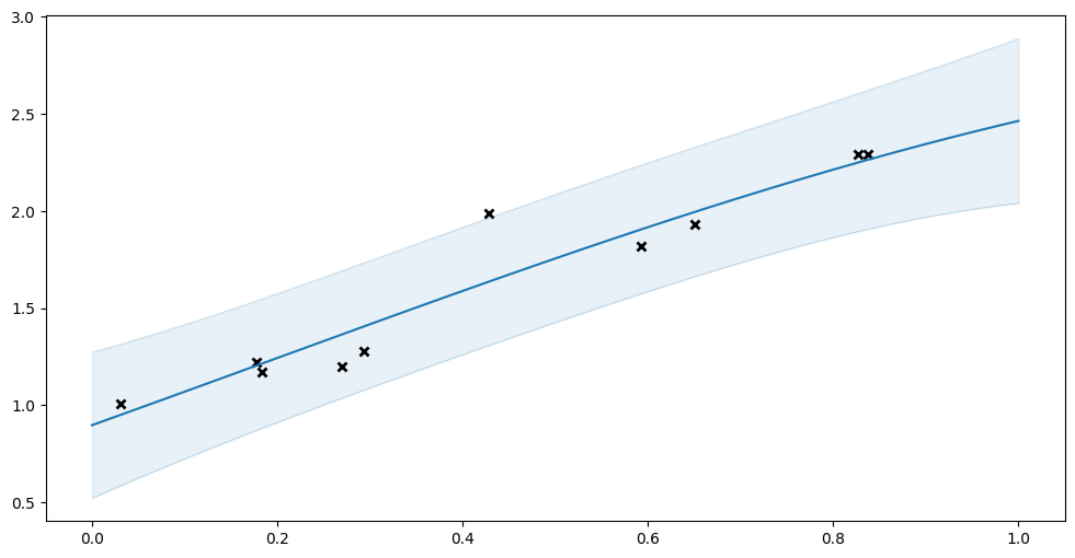
Notice the high variance predicted by the model, and how the model consistently overestimate \(f\) around the non-outlier middle points.

Instead, let us try fitting a VGP with a Student’s t-distribution as likelihood. The Student’s t-distribution has heavier tails, and will be less affected by an outlier.

model = gpflow.models.VGP(
    (X, Y),
    kernel=gpflow.kernels.SquaredExponential(),
    likelihood=gpflow.likelihoods.StudentT(),
)
plot_model(model)

name	class	transform	prior	trainable	shape	dtype	value
VGP.kernel.variance	Parameter	Softplus		True	()	float64	5.04051
VGP.kernel.lengthscales	Parameter	Softplus		True	()	float64	1.2941
VGP.likelihood.scale	Parameter	Softplus + Shift		True	()	float64	0.05425931071105466
VGP.num_data	Parameter	Identity		False	()	int32	10
VGP.q_mu	Parameter	Identity		True	(10, 1)	float64	[[5.16603723e-01...
VGP.q_sqrt	Parameter	FillTriangular		True	(1, 10, 10)	float64	[[[1.31215603e-02, 0.00000000e+00, 0.00000000e+00...

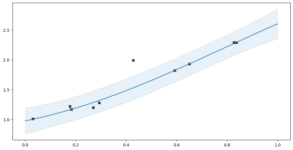
Notice how this fit has smaller uncertainty, and is a much better fit for the non-outlier points.

Classification

Variational models and custom likelihoods allow you to have arbitrary connections beween the data you are modelling and the real-valued function \(f\). For example, we can use it for a classification problem where we are not trying to predict a real value (regression), but trying to predict an object label instead.

To do classification we start with our unknown function \(f\). \(f\) can have any (real) value, but we want to use it for probabilities, so we need to map it to the interval \([0; 1]\). We will use the cumulative density function of a standard normal for this. Other functions can be used for this “squishing”, but the cumulative density function has nice analytical properties that simplifies some maths. We then use the mapped value as the probability in a Bernoulli trial to determine the output class (\(Y\)). All of this is encapsulated in the GPflow Bernoulli class.

Assume we have two sets of points:

X1 = np.array(
    [[0.218], [0.453], [0.196], [0.638], [0.523], [0.541], [0.455], [0.632], [0.309], [0.330]]
)
X2 = np.array(
    [[0.868], [0.706], [0.672], [0.742], [0.813], [0.617], [0.456], [0.838], [0.730], [0.841]]
)

plt.scatter(X1, np.zeros_like(X1))
plt.scatter(X2, np.zeros_like(X2))

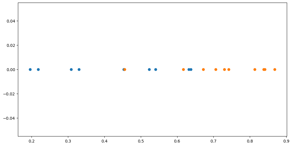
Given a new point, we want to predict which one of those two sets it should belong to.

First we will massage our data into one \((X, Y)\) dataset, instead of two \(X\) datasets. Our \(X\) will be all our points, and our \(Y\) will be either 0 or 1, to signal which one of the two sets the corresponding \(x\) belongs to.

Y1 = np.zeros_like(X1)
Y2 = np.ones_like(X2)
X = np.concatenate([X1, X2], axis=0)
Y = np.concatenate([Y1, Y2], axis=0)

plt.scatter(X, Y)

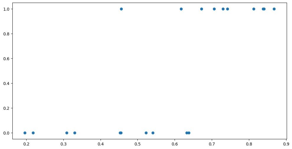
Notice that these are the same points, but instead of using colours, we are using the Y-axis to separate the two sets.

We can train a model on this the usual way:

model = gpflow.models.VGP(
    (X, Y),
    kernel=gpflow.kernels.SquaredExponential(),
    likelihood=gpflow.likelihoods.Bernoulli(),
)
opt = gpflow.optimizers.Scipy()
opt.minimize(model.training_loss, model.trainable_variables)
gpflow.utilities.print_summary(model, "notebook")

name	class	transform	prior	trainable	shape	dtype	value
VGP.kernel.variance	Parameter	Softplus		True	()	float64	4.18082
VGP.kernel.lengthscales	Parameter	Softplus		True	()	float64	0.34062610361649165
VGP.num_data	Parameter	Identity		False	()	int32	20
VGP.q_mu	Parameter	Identity		True	(20, 1)	float64	[[-9.27295579e-01...
VGP.q_sqrt	Parameter	FillTriangular		True	(1, 20, 20)	float64	[[[4.53641708e-01, 0.00000000e+00, 0.00000000e+00...

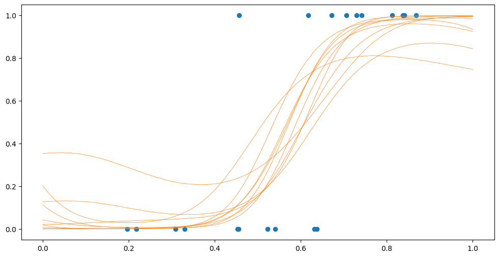
When doing predictions, beware that since we are no longer using a Gaussian likelihood - in fact our likelihood is not even symmetric - it is much harder to make sense of the mean and variance returned by predict_f and predict_y. Instead, let us draw samples of f:

Xplot = np.linspace(0, 1, 200)[:, None]
Fsamples = model.predict_f_samples(Xplot, 10).numpy().squeeze().T

plt.plot(Xplot, Fsamples, "C0", lw=0.5)

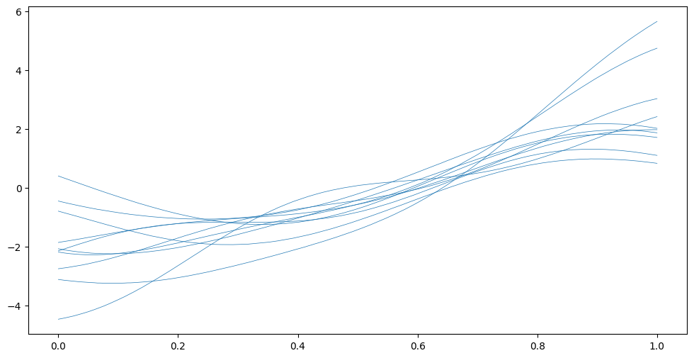
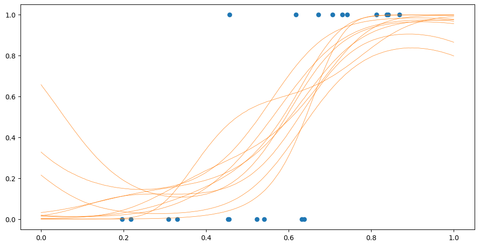
How do we interpret this? Remember these are \(f\) samples from before they’re “squished” into the \([0; 1]\) range. The likelihood.invlink function implements the above-mentioned cumulative density function that is used to perform the “squishing”. We can use this to map our \(f\) samples to probabilities:

Psamples = model.likelihood.invlink(Fsamples)

plt.plot(Xplot, Psamples, "C1", lw=0.5)
plt.scatter(X, Y)

We can use the mean, “squished” through our invlink to get a probability of a point being in group 0:

Fmean, _ = model.predict_f(Xplot)
P = model.likelihood.invlink(Fmean)

plt.plot(Xplot, P, "C1")
plt.scatter(X, Y)

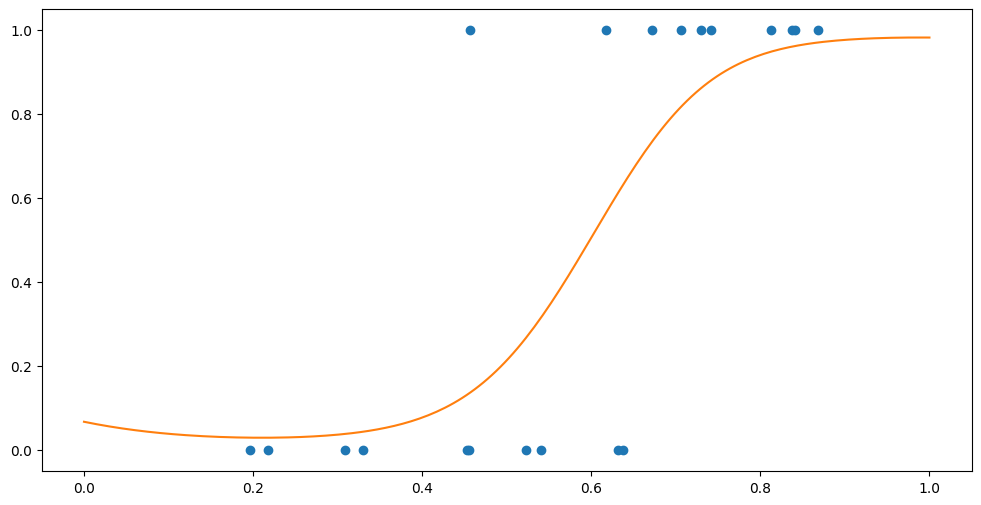
So if we want to predict the class at \(x=0.3\) we would do:

Xnew = np.array([[0.3]])
Fmean, _ = model.predict_f(Xnew)
P = model.likelihood.invlink(Fmean)
P

<tf.Tensor: shape=(1, 1), dtype=float64, numpy=array([[0.03717187]])>

Which mean a \(\sim3.7\%\) chance of class 0, and \(100\% - 3.7\% = 96.3\%\) chance of class 1.

You may also be interested in our advanced tutorial on multiclass classification.

The Sparse Variational Gaussian Process

The Sparse Variational Gaussian Process (SVGP) combines the sparsity we studied in the previous chapter, with the generic likelihoods we have seen in this chapter. It gets a separate section, because its API is slightly different from what we’ve seen before. All the other models we have seen use the InternalDataTrainingLossMixin and internally store their data. The SVGP uses the ExternalDataTrainingLossMixin. This means it does not take its data in the constructor, and instead takes the data as parameters when training the model.

Let us try fitting a SVGP to our classification data:

model = gpflow.models.SVGP(
    kernel=gpflow.kernels.SquaredExponential(),
    likelihood=gpflow.likelihoods.Bernoulli(),
    inducing_variable=np.linspace(0.0, 1.0, 4)[:, None],
)
opt = gpflow.optimizers.Scipy()
opt.minimize(model.training_loss_closure((X, Y)), model.trainable_variables)
gpflow.utilities.print_summary(model, "notebook")

name	class	transform	prior	trainable	shape	dtype	value
SVGP.kernel.variance	Parameter	Softplus		True	()	float64	4.17754
SVGP.kernel.lengthscales	Parameter	Softplus		True	()	float64	0.3406899522682016
SVGP.inducing_variable.Z	Parameter	Identity		True	(4, 1)	float64	[[0.211331...
SVGP.q_mu	Parameter	Identity		True	(4, 1)	float64	[[-0.92779766...
SVGP.q_sqrt	Parameter	FillTriangular		True	(1, 4, 4)	float64	[[[0.46160276, 0., 0....

Notice the parameters provided to the model initialiser, and the parameters passed to model.training_loss_closure.

Let us plot our results:

Fsamples = model.predict_f_samples(Xplot, 10).numpy().squeeze().T
Psamples = model.likelihood.invlink(Fsamples)

plt.plot(Xplot, Psamples, "C1", lw=0.5)
plt.scatter(X, Y)

The combination of external training data and inducing points allow the SVGP to be trained on truly huge datasets. For details, see our advanced tutorial on scalability.

Writing code that handles both internal and external data models

Having some models store training data internally, while others take it as a parameter when training, can be frustrating if you are trying to write code that works with a generic model. The gpflow.models module contains some functions that can help you write generic code.

Here is an example of how one might write a generic model training function:

def train_generic_model(
    model: gpflow.models.GPModel, data: gpflow.base.RegressionData
) -> None:
    loss = gpflow.models.training_loss_closure(model, data)
    opt = gpflow.optimizers.Scipy()
    opt.minimize(loss, model.trainable_variables)

For example, this works with both a VGP and an SVGP:

data = (X, Y)
models: Sequence[gpflow.models.GPModel] = [
    gpflow.models.VGP(
        data,
        kernel=gpflow.kernels.SquaredExponential(),
        likelihood=gpflow.likelihoods.Bernoulli(),
    ),
    gpflow.models.SVGP(
        kernel=gpflow.kernels.SquaredExponential(),
        likelihood=gpflow.likelihoods.Bernoulli(),
        inducing_variable=np.linspace(0.0, 1.0, 4)[:, None],
    ),
]
for model in models:
    train_generic_model(model, data)