Kernels#
In this chapter we will be explaining what kernels are, how they affect your models, and how you can create them.
These are the imports we will be using below:
[1]:
from copy import deepcopy

import matplotlib.pyplot as plt
import numpy as np
import tensorflow as tf
from matplotlib.axes import Axes
from matplotlib.cm import coolwarm

import gpflow
What is a kernel?#
Remember how we assume that our data is generated by:
\begin{equation} Y_i = f(X_i) + \varepsilon_i \,, \quad \varepsilon_i \sim \mathcal{N}(0, \sigma^2). \end{equation}
And in Basic Usage we defined our model as:
[2]:
model = gpflow.models.GPR(
    (X, Y),
    kernel=gpflow.kernels.SquaredExponential(),
)
The kernel defines what kind of shapes \(f\) can take, and it is one of the primary ways you fit your model to your data.
Technically, a kernel is a function that takes \(X\) values and returns a \(N \times N\) covariance matrix telling us how those \(X\) coordinates relate to each other. However, for many users it may be more useful to develop an intuitive understanding of how the different kernels behave than to study the maths.
A kernel is sometimes also known as a covariance function.
Below we will introduce the most important kernels, and how they can be composed to create new kernels that fit any structure in your data. To see the full list of kernels implemented in GPflow vist our API documentation.
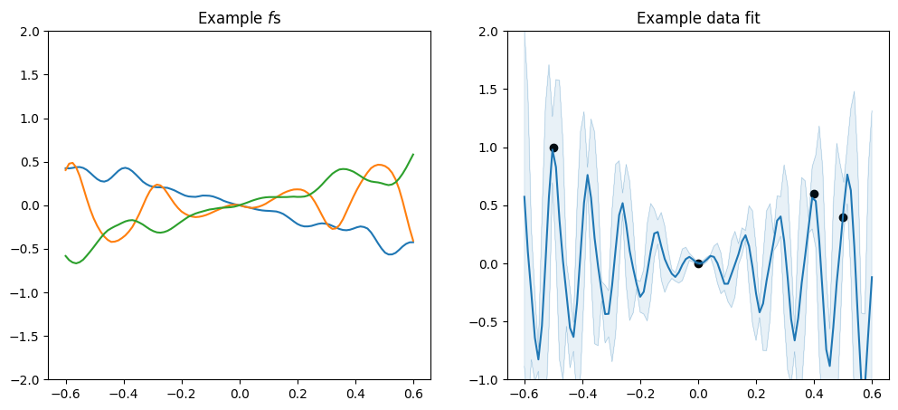
Visualising a kernel#
In this chapter we will investigate many different kernels. To be able to understand a kernel it is helpful to plot some samples from it. So, we will first write a helper function for plotting a kernel:
[3]:
def plot_kernel_samples(ax: Axes, kernel: gpflow.kernels.Kernel) -> None:
    X = np.zeros((0, 1))
    Y = np.zeros((0, 1))
    model = gpflow.models.GPR((X, Y), kernel=deepcopy(kernel))
    Xplot = np.linspace(-0.6, 0.6, 100)[:, None]
    tf.random.set_seed(20220903)
    n_samples = 3
    # predict_f_samples draws n_samples examples of the function f, and returns their values at Xplot.
    fs = model.predict_f_samples(Xplot, n_samples)
    ax.plot(Xplot, fs[:, :, 0].numpy().T, label=kernel.__class__.__name__)
    ax.set_ylim(bottom=-2.0, top=2.0)
    ax.set_title("Example $f$s")


def plot_kernel_prediction(
    ax: Axes, kernel: gpflow.kernels.Kernel, *, optimise: bool = True
) -> None:
    X = np.array([[-0.5], [0.0], [0.4], [0.5]])
    Y = np.array([[1.0], [0.0], [0.6], [0.4]])
    model = gpflow.models.GPR(
        (X, Y), kernel=deepcopy(kernel), noise_variance=1e-3
    )

    if optimise:
        gpflow.set_trainable(model.likelihood, False)
        opt = gpflow.optimizers.Scipy()
        opt.minimize(model.training_loss, model.trainable_variables)

    Xplot = np.linspace(-0.6, 0.6, 100)[:, None]

    f_mean, f_var = model.predict_f(Xplot, full_cov=False)
    f_lower = f_mean - 1.96 * np.sqrt(f_var)
    f_upper = f_mean + 1.96 * np.sqrt(f_var)

    ax.scatter(X, Y, color="black")
    (mean_line,) = ax.plot(Xplot, f_mean, "-", label=kernel.__class__.__name__)
    color = mean_line.get_color()
    ax.plot(Xplot, f_lower, lw=0.1, color=color)
    ax.plot(Xplot, f_upper, lw=0.1, color=color)
    ax.fill_between(
        Xplot[:, 0], f_lower[:, 0], f_upper[:, 0], color=color, alpha=0.1
    )
    ax.set_ylim(bottom=-1.0, top=2.0)
    ax.set_title("Example data fit")


def plot_kernel(
    kernel: gpflow.kernels.Kernel, *, optimise: bool = True
) -> None:
    _, (samples_ax, prediction_ax) = plt.subplots(nrows=1, ncols=2)
    plot_kernel_samples(samples_ax, kernel)
    plot_kernel_prediction(prediction_ax, kernel, optimise=optimise)
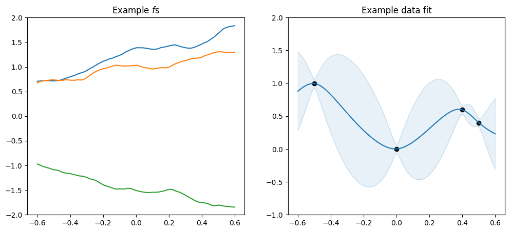
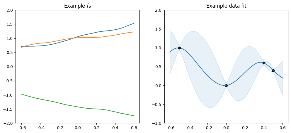
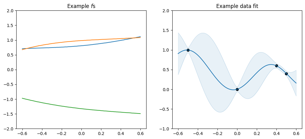
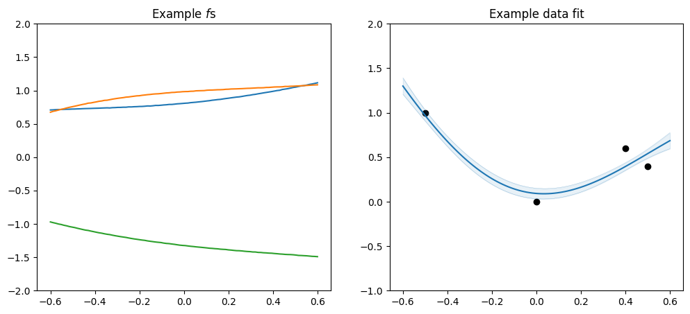
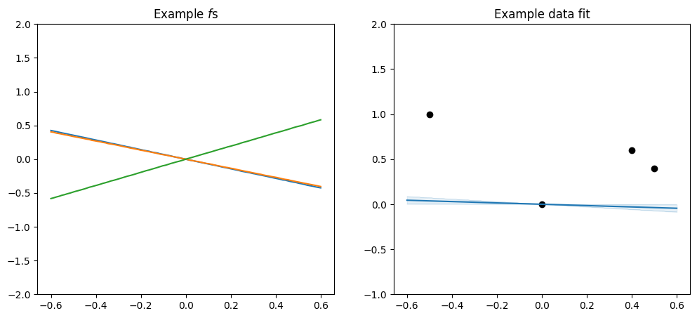
The Matérn family#
The Matérn family of kernels covers the most popular and widely used kernels.
A Matérn kernel has a parameter called \(\nu\), which determines the smoothness of \(f\) - the higher the \(\nu\), the smoother \(f\). The maths of the kernels simplifies significantly when \(\nu\) is one of \(\frac{1}{2}\), \(\frac{3}{2}\), \(\frac{5}{2}\), etc., so those are the ones usually used in practice. As \(\nu\) diverges towards \(\infty\), we recover the squared exponential kernel we used in Basic Usage.
GPflow implements the following kernels from the Matérn family:
Matern12Matern32Matern52SquaredExponential
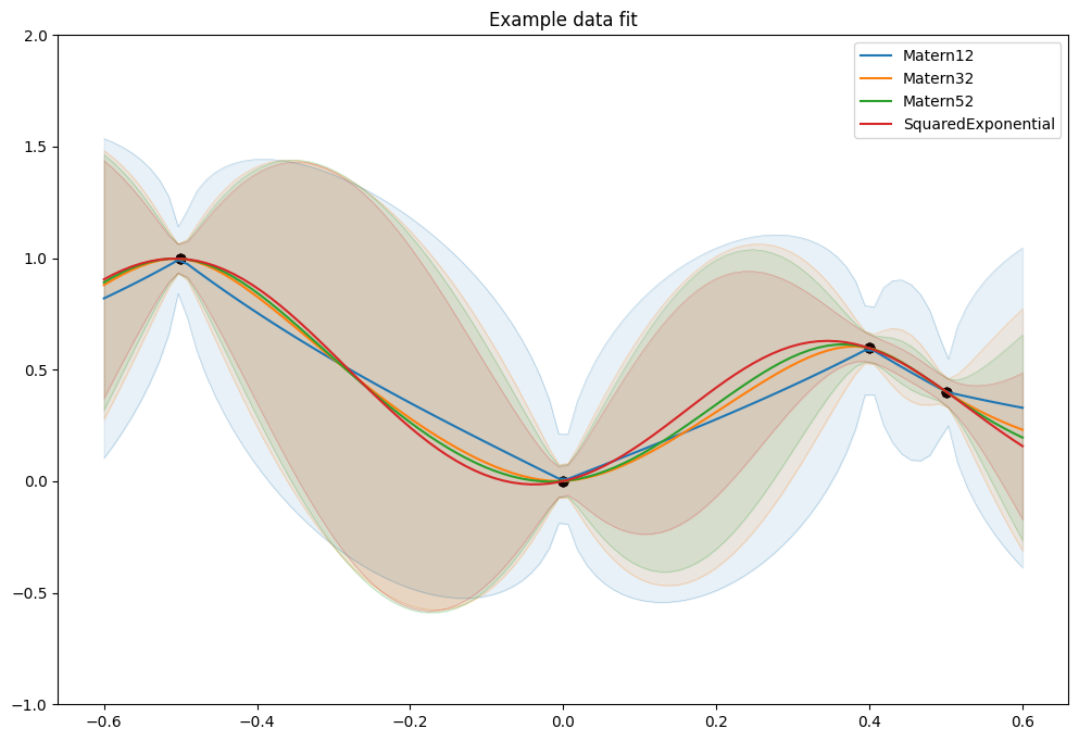
As mentioned above the \(\nu\) parameter determines smoothnes, and in particular a SquaredExponential kernel will infer an \(f\) that is infinitely many times differentiable, a Matern52 an \(f\) that is twice differentiable, a Matern32 an \(f\) that is once differentiable, and a Matern12 an \(f\) that is not differentiable.
Note that the squared exponential kernel is also sometimes known as the SE-, radial basis function-, RBF-, or exponentiated quadratic kernel.
Let’s look at some samples:
[4]:
plot_kernel(gpflow.kernels.Matern12())
[5]:
plot_kernel(gpflow.kernels.Matern32())
[6]:
plot_kernel(gpflow.kernels.Matern52())
[7]:
plot_kernel(gpflow.kernels.SquaredExponential())
And all of them together:
[8]:
_, ax = plt.subplots(nrows=1, ncols=1)
plot_kernel_prediction(ax, gpflow.kernels.Matern12())
plot_kernel_prediction(ax, gpflow.kernels.Matern32())
plot_kernel_prediction(ax, gpflow.kernels.Matern52())
plot_kernel_prediction(ax, gpflow.kernels.SquaredExponential())
ax.legend()
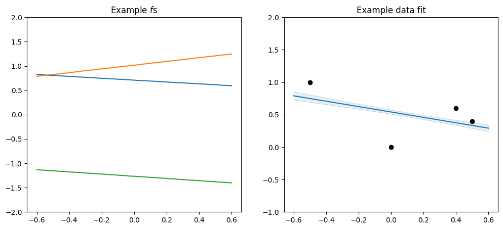
Kernel parameters#
The kernel classes generally have parameters that can affect the shape of \(f\).
For example, all the Matérn family kernels mentioned above have two parameters:
variance, which determines the scale along the \(y\) axis, andlengthscales, which determines the scale along the \(x\) axis.
For example:
[9]:
plot_kernel(
    gpflow.kernels.SquaredExponential(variance=0.1, lengthscales=0.2),
    optimise=False,
)
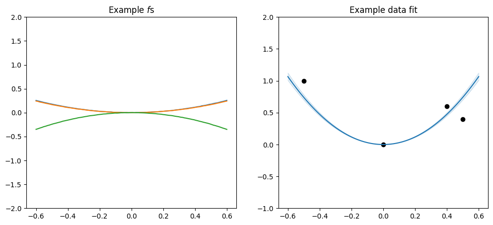
[10]:
plot_kernel(
    gpflow.kernels.SquaredExponential(variance=1.0, lengthscales=0.2),
    optimise=False,
)
[11]:
plot_kernel(
    gpflow.kernels.SquaredExponential(variance=1.0, lengthscales=1.0),
    optimise=False,
)
These parameters are usually set automatically during model training, and ideally you don’t need to worry too much about them. In the above examples we did not optimise the model, to demonstrate how model parameters impact predictions. For more about parameters and their training see our section on Parameters and Their Optimisation.
To see which parameters each kernel takes, look up their API documentation.
Kernel composition#
Often you can just pick an appropriate Matérn kernel, train it, and you will have a reasonable model.
However, if you need more performance from your model, and if your data has interesting structure, you can create a new kernel tailored specifically for your problem.
You can create a new kernel from the bottom up by extending the `gpflow.kernels.Kernel class <../../api/gpflow/kernels/index.rst#gpflow-kernels-kernel>`__, but that is advanced usage, and we are not going to demonstrate that here.
A much easier way to get a tailored kernel is to combine existing ones, and we demonstrate how to do that below.
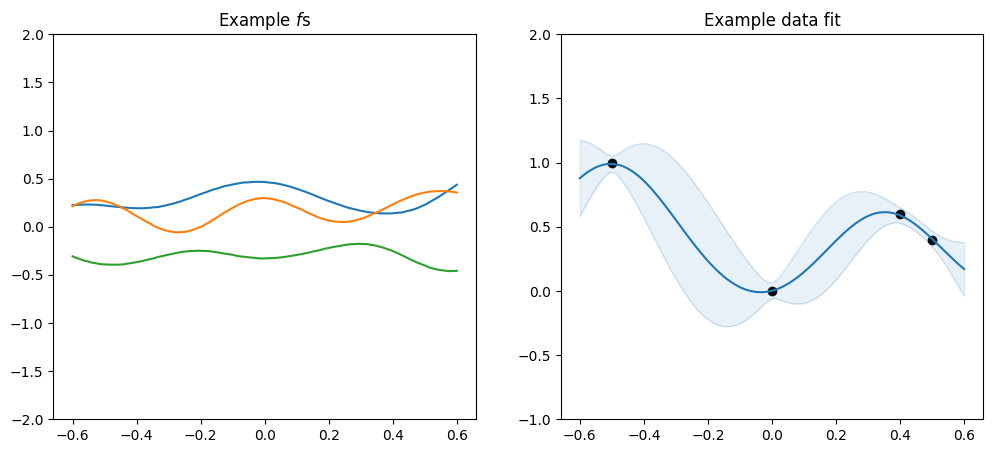
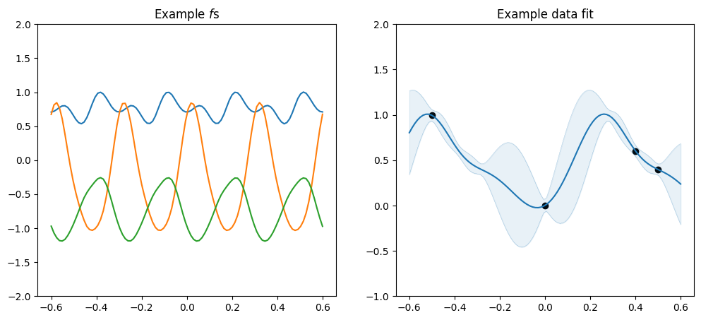
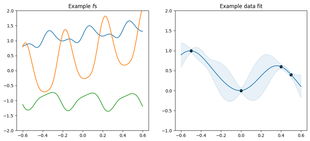
Periodic#
The Periodic kernel is a composite kernel that wraps another kernel, and creates a version that repeats:
[12]:
plot_kernel(
    gpflow.kernels.Periodic(gpflow.kernels.SquaredExponential(), period=0.3)
)
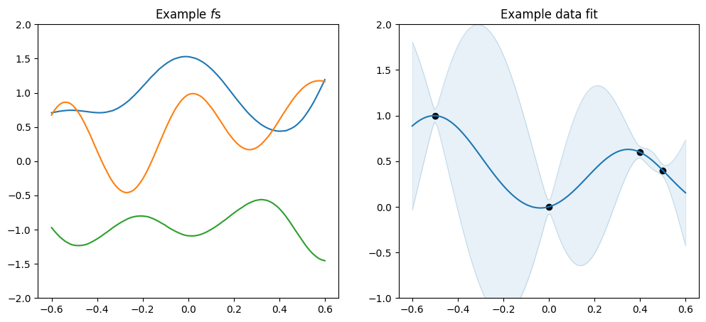
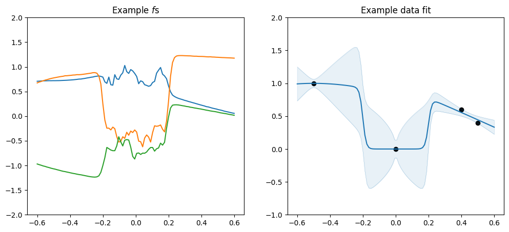
Change-points#
The ChangePoints kernel allows you to use different \(f\)s for different regions of \(X\). The kernels parameter determines which kernels to use, and the locations parameter determines where to switch between the kernels. steepness sets how rapid the transitions between the \(f\)s are.
[13]:
plot_kernel(
    gpflow.kernels.ChangePoints(
        kernels=[
            gpflow.kernels.Matern52(lengthscales=1.0),
            gpflow.kernels.Matern12(lengthscales=3.0),
            gpflow.kernels.SquaredExponential(lengthscales=2.0),
        ],
        locations=[-0.2, 0.2],
        steepness=100.0,
    ),
    optimise=False,
)
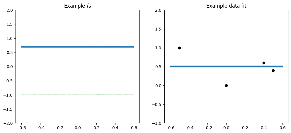
Some other simple kernels#
Before we continue, I want to introduce a couple of simple kernels that rarely are used alone, but makes it easy to demonstrate some other concepts below.
We have the Constant kernel, which makes \(f\) a constant value:
[14]:
plot_kernel(gpflow.kernels.Constant())
And we have the Linear kernel, which creates a stright line through \((0, 0)\):
[15]:
plot_kernel(gpflow.kernels.Linear())
Addition and multiplication#
Other than the kernels that explicitly takes other kernels as parameters, you can compose kernels with the + and * binary operators. Beware that this adds and multiplies the covariance matrices returned by the kernels, which does not necessarly have an intuitive effect on the \(f\) function that is generated by the kernel.
For example you can add a constant and a linear to get a \(f\) that is a straight line that does not pass through \((0, 0)\):
[16]:
plot_kernel(gpflow.kernels.Linear() + gpflow.kernels.Constant())
Or you can add a linear and a periodic kernel to get repeating pattern with a linear trend:
[17]:
plot_kernel(
    gpflow.kernels.Periodic(gpflow.kernels.SquaredExponential(), period=0.4)
    + gpflow.kernels.Linear()
)
You can multiply two linear kernels to get a quadratic (though please use `gpflow.kernels.Polynomial <../../api/gpflow/kernels/index.rst#gpflow-kernels-polynomial>`__ if you actually want a quadratic function):
[18]:
plot_kernel(gpflow.kernels.Linear() * gpflow.kernels.Linear())
Or you can scale a periodic by a linear:
[19]:
plot_kernel(
    gpflow.kernels.Periodic(gpflow.kernels.SquaredExponential(), period=0.3)
    * gpflow.kernels.Linear()
)
Multiple-dimensional data#
So far we’ve been using 1D input and 1D output data, because it’s easy to understand and to plot.
However, with real data you often have multiple input dimensions, or even output dimensions.
GPflow has great support for multiple input dimensions. When you have multiple input dimensions it is interesting how \(f\) behaves along every one of those dimensions, and hence it is interesting how your kernel handles each dimension.
Working with multiple output dimensions is more complicated. We have a guide on how to do this in a principled way, but be aware that this is an advanced topic.
Let us define a function to plot a kernel with 2D input:
[20]:
def plot_2d_kernel_samples(ax: Axes, kernel: gpflow.kernels.Kernel) -> None:
    n_grid = 30
    X = np.zeros((0, 2))
    Y = np.zeros((0, 1))
    model = gpflow.models.GPR((X, Y), kernel=deepcopy(kernel))

    Xplots = np.linspace(-0.6, 0.6, n_grid)
    Xplot1, Xplot2 = np.meshgrid(Xplots, Xplots)
    Xplot = np.stack([Xplot1, Xplot2], axis=-1)
    Xplot = Xplot.reshape([n_grid ** 2, 2])

    tf.random.set_seed(20220903)
    fs = model.predict_f_samples(Xplot, num_samples=1)
    fs = fs.numpy().reshape((n_grid, n_grid))
    ax.plot_surface(Xplot1, Xplot2, fs, cmap=coolwarm)
    ax.set_title("Example $f$")


def plot_2d_kernel_prediction(ax: Axes, kernel: gpflow.kernels.Kernel) -> None:
    n_grid = 30
    # hide: begin
    # fmt: off
    # hide: end
    X = np.array(
        [
            [-0.4, -0.5], [0.1, -0.3], [0.4, -0.4], [0.5, -0.5], [-0.5, 0.3],
            [0.0, 0.5], [0.4, 0.4], [0.5, 0.3],
        ]
    )
    Y = np.array([[0.8], [0.0], [0.5], [0.3], [1.0], [0.2], [0.7], [0.5]])
    # hide: begin
    # fmt: on
    # hide: end
    model = gpflow.models.GPR(
        (X, Y), kernel=deepcopy(kernel), noise_variance=1e-3
    )
    gpflow.set_trainable(model.likelihood, False)
    opt = gpflow.optimizers.Scipy()
    opt.minimize(model.training_loss, model.trainable_variables)

    Xplots = np.linspace(-0.6, 0.6, n_grid)
    Xplot1, Xplot2 = np.meshgrid(Xplots, Xplots)
    Xplot = np.stack([Xplot1, Xplot2], axis=-1)
    Xplot = Xplot.reshape([n_grid ** 2, 2])

    f_mean, _ = model.predict_f(Xplot, full_cov=False)
    f_mean = f_mean.numpy().reshape((n_grid, n_grid))
    ax.plot_surface(Xplot1, Xplot2, f_mean, cmap=coolwarm, alpha=0.7)
    ax.scatter(X[:, 0], X[:, 1], Y[:, 0], s=50, c="black")
    ax.set_title("Example data fit")


def plot_2d_kernel(kernel: gpflow.kernels.Kernel) -> None:
    _, (samples_ax, prediction_ax) = plt.subplots(
        nrows=1, ncols=2, subplot_kw={"projection": "3d"}
    )
    plot_2d_kernel_samples(samples_ax, kernel)
    plot_2d_kernel_prediction(prediction_ax, kernel)
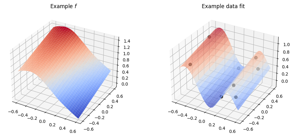
Now, if we just use a kernel with default parameters, like we did above, with multi-dimensional input data it will work:
[21]:
plot_2d_kernel(gpflow.kernels.SquaredExponential())
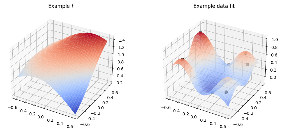
However, by default the kernel will use the same parameters for all the input dimensions, and in practice it is rare that all the input dimensions behave in the same way, so usually this is not what we want.
Multi-dimensional parameters#
Many kernels allow relevant parameters to be a vector of values, one for each input dimension, instead of just a single value. This is an easy way to have a kernel that behaves differently for each input dimension.
To use this, initialise the parameter to a vector with one entry per input dimension:
[22]:
plot_2d_kernel(gpflow.kernels.SquaredExponential(lengthscales=[0.1, 0.5]))
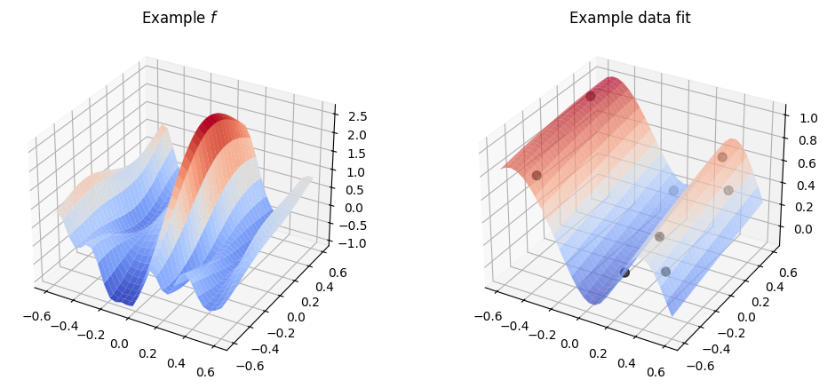
Notice that even though we explicitly initialise the lengthscales the values are still optimised / scaled, so usually you do not have to worry too much about setting the values right.
Again, see our section on Parameters and Their Optimisation to better understand how parameters are set and trained.
Active dimensions#
Another way to customise kernel behavior along different dimensions is “active dimensions”. Most kernels take an argument active_dims that determines which input dimensions that kernel cares about. The kernel will simply ignore input dimensions not listed in active_dims. You can combine this with + addition of kernels to create a kernel that has specific behaviour along each dimension:
[23]:
plot_2d_kernel(
    gpflow.kernels.Matern52(active_dims=[0])
    + gpflow.kernels.Linear(active_dims=[1])
)