MCMC (Markov Chain Monte Carlo)
GPflow allows you to approximate the posterior over the latent functions of its models (and over the hyperparemeters after setting a prior for those) using Hamiltonian Monte Carlo (HMC)
[1]:
import numpy as np
import matplotlib.pyplot as plt
import tensorflow as tf
import tensorflow_probability as tfp
from tensorflow_probability import distributions as tfd

import gpflow
from gpflow.ci_utils import ci_niter
from gpflow import set_trainable
from multiclass_classification import plot_from_samples, colors

gpflow.config.set_default_float(np.float64)
gpflow.config.set_default_jitter(1e-4)
gpflow.config.set_default_summary_fmt("notebook")
# convert to float64 for tfp to play nicely with gpflow in 64
f64 = gpflow.utilities.to_default_float

tf.random.set_seed(123)


%matplotlib inline
In this notebook, we provide three examples:
Example 1: Sampling hyperparameters in Gaussian process regression
Example 2: Sparse Variational MC applied to the multiclass classification problem
Example 3: Full Bayesian inference for Gaussian process models
Example 1: GP regression
We first consider the GP regression (with Gaussian noise) for which the marginal likelihood \(p(\mathbf y\,|\,\theta)\) can be computed exactly.
The GPR model parameterized by \(\theta = [\tau]\) is given by
where \(f \sim \mathcal{GP}(\mu(.), k(., .))\), and \(\varepsilon \sim \mathcal{N}(0, \tau^2 I)\).
See the Basic (Gaussian likelihood) GP regression model for more details on GPR and for a treatment of the direct likelihood maximization.
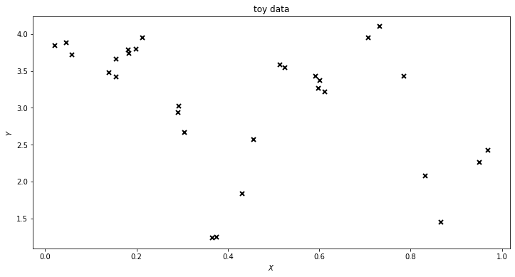
Data for a one-dimensional regression problem
[2]:
rng = np.random.RandomState(42)

N = 30


def synthetic_data(num: int, rng: np.random.RandomState):
    X = rng.rand(num, 1)
    Y = np.sin(12 * X) + 0.66 * np.cos(25 * X) + rng.randn(num, 1) * 0.1 + 3
    return X, Y


data = (X, Y) = synthetic_data(N, rng)

plt.figure(figsize=(12, 6))
plt.plot(X, Y, "kx", mew=2)
plt.xlabel("$X$")
plt.ylabel("$Y$")
plt.title("toy data")
plt.show()
MCMC for hyperparameters \(\theta\)
We now want to sample from the posterior over \(\theta\):
Firstly, we build the GPR model.
[3]:
kernel = gpflow.kernels.Matern52(lengthscales=0.3)
mean_function = gpflow.mean_functions.Linear(1.0, 0.0)
model = gpflow.models.GPR(data, kernel, mean_function, noise_variance=0.01)
2022-03-18 10:07:26.295276: I tensorflow/stream_executor/cuda/cuda_gpu_executor.cc:936] successful NUMA node read from SysFS had negative value (-1), but there must be at least one NUMA node, so returning NUMA node zero
2022-03-18 10:07:26.298667: W tensorflow/stream_executor/platform/default/dso_loader.cc:64] Could not load dynamic library 'libcusolver.so.11'; dlerror: libcusolver.so.11: cannot open shared object file: No such file or directory
2022-03-18 10:07:26.299228: W tensorflow/core/common_runtime/gpu/gpu_device.cc:1850] Cannot dlopen some GPU libraries. Please make sure the missing libraries mentioned above are installed properly if you would like to use GPU. Follow the guide at https://www.tensorflow.org/install/gpu for how to download and setup the required libraries for your platform.
Skipping registering GPU devices...
2022-03-18 10:07:26.299751: I tensorflow/core/platform/cpu_feature_guard.cc:151] This TensorFlow binary is optimized with oneAPI Deep Neural Network Library (oneDNN) to use the following CPU instructions in performance-critical operations:  AVX2 FMA
To enable them in other operations, rebuild TensorFlow with the appropriate compiler flags.
Secondly, we initialize the model to the maximum likelihood solution.
[4]:
optimizer = gpflow.optimizers.Scipy()
optimizer.minimize(model.training_loss, model.trainable_variables)

print(f"log posterior density at optimum: {model.log_posterior_density()}")
2022-03-18 10:07:26.325122: W tensorflow/python/util/util.cc:368] Sets are not currently considered sequences, but this may change in the future, so consider avoiding using them.
log posterior density at optimum: -2.437136697069384
Thirdly, we add priors to the hyperparameters.
[5]:
# tfp.distributions dtype is inferred from parameters - so convert to 64-bit
model.kernel.lengthscales.prior = tfd.Gamma(f64(1.0), f64(1.0))
model.kernel.variance.prior = tfd.Gamma(f64(1.0), f64(1.0))
model.likelihood.variance.prior = tfd.Gamma(f64(1.0), f64(1.0))
model.mean_function.A.prior = tfd.Normal(f64(0.0), f64(10.0))
model.mean_function.b.prior = tfd.Normal(f64(0.0), f64(10.0))

gpflow.utilities.print_summary(model)
| name | class | transform | prior | trainable | shape | dtype | value |
|---|---|---|---|---|---|---|---|
| GPR.mean_function.A | Parameter | Identity | Normal | True | (1, 1) | float64 | [[-1.06377032]] |
| GPR.mean_function.b | Parameter | Identity | Normal | True | () | float64 | 3.54746034440109 |
| GPR.kernel.variance | Parameter | Softplus | Gamma | True | () | float64 | 0.9357531803029687 |
| GPR.kernel.lengthscales | Parameter | Softplus | Gamma | True | () | float64 | 0.10390237142109285 |
| GPR.likelihood.variance | Parameter | Softplus + Shift | Gamma | True | () | float64 | 0.005756764054346137 |
We now sample from the posterior using HMC.
[6]:
num_burnin_steps = ci_niter(300)
num_samples = ci_niter(500)

# Note that here we need model.trainable_parameters, not trainable_variables - only parameters can have priors!
hmc_helper = gpflow.optimizers.SamplingHelper(
    model.log_posterior_density, model.trainable_parameters
)

hmc = tfp.mcmc.HamiltonianMonteCarlo(
    target_log_prob_fn=hmc_helper.target_log_prob_fn, num_leapfrog_steps=10, step_size=0.01
)
adaptive_hmc = tfp.mcmc.SimpleStepSizeAdaptation(
    hmc, num_adaptation_steps=10, target_accept_prob=f64(0.75), adaptation_rate=0.1
)


@tf.function
def run_chain_fn():
    return tfp.mcmc.sample_chain(
        num_results=num_samples,
        num_burnin_steps=num_burnin_steps,
        current_state=hmc_helper.current_state,
        kernel=adaptive_hmc,
        trace_fn=lambda _, pkr: pkr.inner_results.is_accepted,
    )


samples, traces = run_chain_fn()
parameter_samples = hmc_helper.convert_to_constrained_values(samples)

param_to_name = {param: name for name, param in gpflow.utilities.parameter_dict(model).items()}
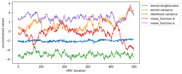
NOTE: All the Hamiltonian MCMC sampling takes place in an unconstrained space (where constrained parameters have been mapped via a bijector to an unconstrained space). This makes the optimization, as required in the gradient step, much easier.
However, we often wish to sample the constrained parameter values, not the unconstrained one. The SamplingHelper helps us convert our unconstrained values to constrained parameter ones.
[7]:
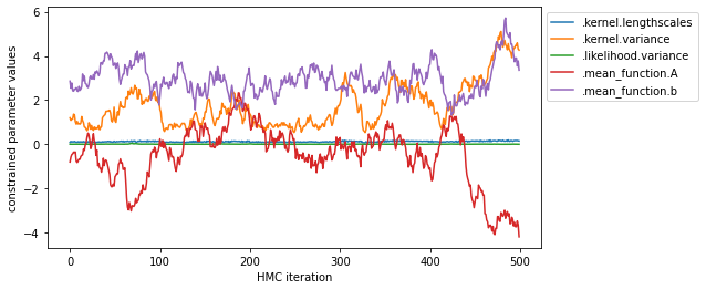
def plot_samples(samples, parameters, y_axis_label):
    plt.figure(figsize=(8, 4))
    for val, param in zip(samples, parameters):
        plt.plot(tf.squeeze(val), label=param_to_name[param])
    plt.legend(bbox_to_anchor=(1.0, 1.0))
    plt.xlabel("HMC iteration")
    plt.ylabel(y_axis_label)


plot_samples(samples, model.trainable_parameters, "unconstrained values")
plot_samples(parameter_samples, model.trainable_parameters, "constrained parameter values")
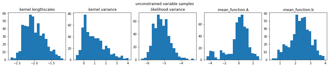
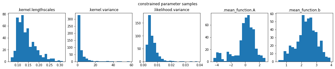
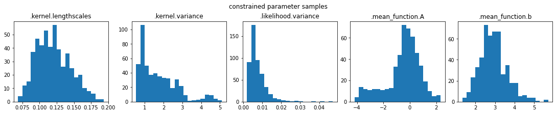
You can also inspect the marginal distribution of samples.
[8]:
def marginal_samples(samples, parameters, y_axis_label):
    fig, axes = plt.subplots(1, len(param_to_name), figsize=(15, 3), constrained_layout=True)
    for ax, val, param in zip(axes, samples, parameters):
        ax.hist(np.stack(val).flatten(), bins=20)
        ax.set_title(param_to_name[param])
    fig.suptitle(y_axis_label)
    plt.show()


marginal_samples(samples, model.trainable_parameters, "unconstrained variable samples")
marginal_samples(parameter_samples, model.trainable_parameters, "constrained parameter samples")
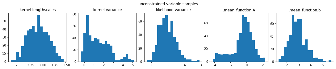
NOTE: The sampler runs in unconstrained space (so that positive parameters remain positive, and parameters that are not trainable are ignored).
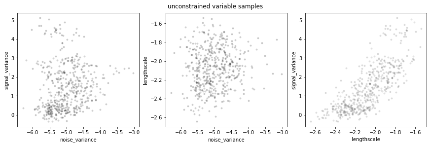
For serious analysis you most certainly want to run the sampler longer, with multiple chains and convergence checks. This will do for illustration though!
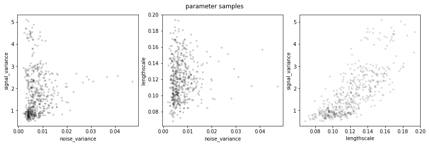
[9]:
def plot_joint_marginals(samples, parameters, y_axis_label):
    name_to_index = {param_to_name[param]: i for i, param in enumerate(parameters)}
    f, axs = plt.subplots(1, 3, figsize=(12, 4), constrained_layout=True)

    axs[0].plot(
        samples[name_to_index[".likelihood.variance"]],
        samples[name_to_index[".kernel.variance"]],
        "k.",
        alpha=0.15,
    )
    axs[0].set_xlabel("noise_variance")
    axs[0].set_ylabel("signal_variance")

    axs[1].plot(
        samples[name_to_index[".likelihood.variance"]],
        samples[name_to_index[".kernel.lengthscales"]],
        "k.",
        alpha=0.15,
    )
    axs[1].set_xlabel("noise_variance")
    axs[1].set_ylabel("lengthscale")

    axs[2].plot(
        samples[name_to_index[".kernel.lengthscales"]],
        samples[name_to_index[".kernel.variance"]],
        "k.",
        alpha=0.1,
    )
    axs[2].set_xlabel("lengthscale")
    axs[2].set_ylabel("signal_variance")
    f.suptitle(y_axis_label)
    plt.show()


plot_joint_marginals(samples, model.trainable_parameters, "unconstrained variable samples")
plot_joint_marginals(parameter_samples, model.trainable_parameters, "parameter samples")
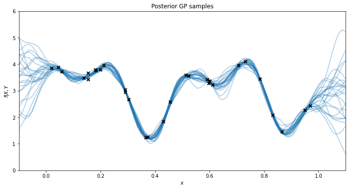
To plot the posterior of predictions, we’ll iterate through the samples and set the model state with each sample. Then, for that state (set of hyperparameters) we’ll draw some samples from the prediction function.
[10]:
# plot the function posterior
xx = np.linspace(-0.1, 1.1, 100)[:, None]
plt.figure(figsize=(12, 6))

for i in range(0, num_samples, 20):
    for var, var_samples in zip(hmc_helper.current_state, samples):
        var.assign(var_samples[i])
    f = model.predict_f_samples(xx, 1)
    plt.plot(xx, f[0, :, :], "C0", lw=2, alpha=0.3)

plt.plot(X, Y, "kx", mew=2)
_ = plt.xlim(xx.min(), xx.max())
_ = plt.ylim(0, 6)
plt.xlabel("$x$")
plt.ylabel("$f|X,Y$")
plt.title("Posterior GP samples")

plt.show()
Example 2: Sparse MC for multiclass classification
We now consider the multiclass classification problem (see the Multiclass classification notebook). Here the marginal likelihood is not available in closed form. Instead we use a sparse variational approximation where we approximate the posterior for each GP as \(q(f_c) \propto p(f_c|\mathbf{u}_c)q(\mathbf{u}_c)\)
In the standard Sparse Variational GP (SVGP) formulation, \(q(\mathbf{u_c})\) is parameterized as a multivariate Gaussian.
An alternative is to directly sample from the optimal \(q(\mathbf{u}_c)\); this is what Sparse Variational GP using MCMC (SGPMC) does.
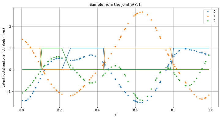
We first build a multiclass classification dataset.
[11]:
# Generate data by sampling from SquaredExponential kernel, and classifying with the argmax
rng = np.random.RandomState(42)

C, N = 3, 100
X = rng.rand(N, 1)
kernel = gpflow.kernels.SquaredExponential(lengthscales=0.1)
K = kernel.K(X) + np.eye(N) * 1e-6

f = rng.multivariate_normal(mean=np.zeros(N), cov=K, size=(C)).T
Y = np.argmax(f, 1).flatten().astype(int)
# One-hot encoding
Y_hot = np.zeros((N, C), dtype=bool)
Y_hot[np.arange(N), Y] = 1

data = (X, Y)
[12]:
plt.figure(figsize=(12, 6))
order = np.argsort(X.flatten())

for c in range(C):
    plt.plot(X[order], f[order, c], ".", color=colors[c], label=str(c))
    plt.plot(X[order], Y_hot[order, c], "-", color=colors[c])

plt.legend()
plt.xlabel("$X$")
plt.ylabel("Latent (dots) and one-hot labels (lines)")
plt.title("Sample from the joint $p(Y, \mathbf{f})$")
plt.grid()
plt.show()
We then build the SGPMC model.
[13]:
kernel = gpflow.kernels.Matern32(lengthscales=0.1) + gpflow.kernels.White(variance=0.01)

model = gpflow.models.SGPMC(
    data,
    kernel=kernel,
    likelihood=gpflow.likelihoods.MultiClass(3),
    inducing_variable=X[::5].copy(),
    num_latent_gps=3,
)
model.kernel.kernels[0].variance.prior = tfd.Gamma(f64(1.0), f64(1.0))
model.kernel.kernels[0].lengthscales.prior = tfd.Gamma(f64(2.0), f64(2.0))
set_trainable(model.kernel.kernels[1].variance, False)

gpflow.utilities.print_summary(model)
| name | class | transform | prior | trainable | shape | dtype | value |
|---|---|---|---|---|---|---|---|
| SGPMC.kernel.kernels[0].variance | Parameter | Softplus | Gamma | True | () | float64 | 1.0 |
| SGPMC.kernel.kernels[0].lengthscales | Parameter | Softplus | Gamma | True | () | float64 | 0.10000000000000002 |
| SGPMC.kernel.kernels[1].variance | Parameter | Softplus | False | () | float64 | 0.009999999999999998 | |
| SGPMC.likelihood.invlink.epsilon | Parameter | Sigmoid | Beta | False | () | float64 | 0.0010000000000000005 |
| SGPMC.inducing_variable.Z | Parameter | Identity | True | (20, 1) | float64 | [[0.37454012... | |
| SGPMC.V | Parameter | Identity | Normal | True | (20, 3) | float64 | [[0., 0., 0.... |
[14]:
# The inducing point locations Z should not be included in the MCMC (see [Hensman et al. (2015)](https://papers.nips.cc/paper/5875-mcmc-for-variationally-sparse-gaussian-processes), hence we set them to non-trainable.
set_trainable(model.inducing_variable, False)
The chain of samples for \(\mathbf{u}_c, \theta\) is initialized at the value maximizing \(p(Y|\mathbf{u}_c, \theta)\).
[15]:
optimizer = gpflow.optimizers.Scipy()
optimizer.minimize(model.training_loss, model.trainable_variables, options={"maxiter": 20})
print(f"log posterior density at optimum: {model.log_posterior_density()}")
log posterior density at optimum: -79.76549027487789
Sampling starts with a ‘burn in’ period.
[16]:
num_burnin_steps = ci_niter(100)
num_samples = ci_niter(500)

# Note that here we need model.trainable_parameters, not trainable_variables - only parameters can have priors!
hmc_helper = gpflow.optimizers.SamplingHelper(
    model.log_posterior_density, model.trainable_parameters
)

hmc = tfp.mcmc.HamiltonianMonteCarlo(
    target_log_prob_fn=hmc_helper.target_log_prob_fn, num_leapfrog_steps=10, step_size=0.01
)

adaptive_hmc = tfp.mcmc.SimpleStepSizeAdaptation(
    hmc, num_adaptation_steps=10, target_accept_prob=f64(0.75), adaptation_rate=0.1
)


@tf.function
def run_chain_fn():
    return tfp.mcmc.sample_chain(
        num_results=num_samples,
        num_burnin_steps=num_burnin_steps,
        current_state=hmc_helper.current_state,
        kernel=adaptive_hmc,
        trace_fn=lambda _, pkr: pkr.inner_results.is_accepted,
    )


samples, _ = run_chain_fn()
constrained_samples = hmc_helper.convert_to_constrained_values(samples)
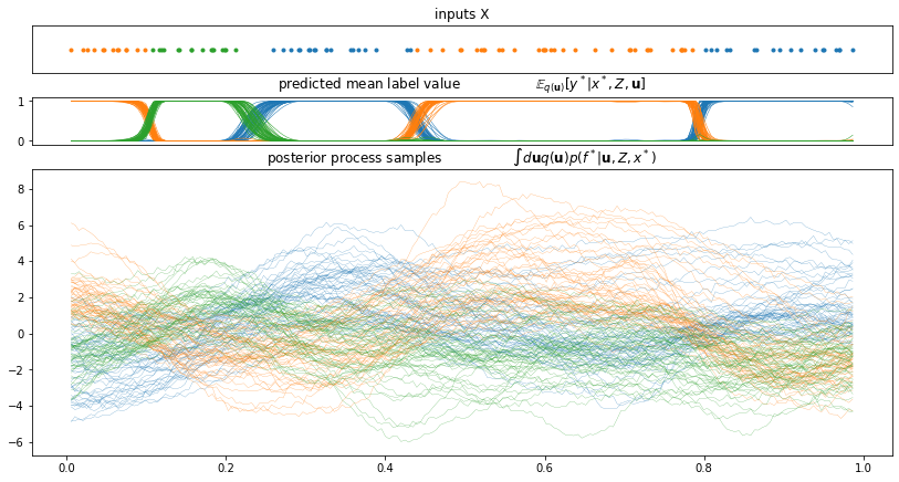
Statistics of the posterior samples can now be reported.
[17]:
plot_from_samples(model, X, Y, model.trainable_parameters, constrained_samples, thin=10)
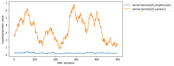
You can also display the sequence of sampled hyperparameters.
[18]:
param_to_name = {param: name for name, param in gpflow.utilities.parameter_dict(model).items()}
name_to_index = {param_to_name[param]: i for i, param in enumerate(model.trainable_parameters)}
hyperparameters = [".kernel.kernels[0].lengthscales", ".kernel.kernels[0].variance"]

plt.figure(figsize=(8, 4))
for param_name in hyperparameters:
    plt.plot(constrained_samples[name_to_index[param_name]], label=param_name)
plt.legend(bbox_to_anchor=(1.0, 1.0))
plt.xlabel("HMC iteration")
_ = plt.ylabel("hyperparameter value")
Example 3: Fully Bayesian inference for generalized GP models with HMC
You can construct very flexible models with Gaussian processes by combining them with different likelihoods (sometimes called ‘families’ in the GLM literature). This makes inference of the GP intractable because the likelihoods are not generally conjugate to the Gaussian process. The general form of the model is
To perform inference in this model, we’ll run MCMC using Hamiltonian Monte Carlo (HMC) over the function values and the parameters \(\theta\) jointly. The key to an effective scheme is rotation of the field using the Cholesky decomposition. We write:
Joint HMC over \(v\) and the function values is not widely adopted in the literature because of the difficulty in differentiating \(LL^\top=K\). We’ve made this derivative available in TensorFlow, and so application of HMC is relatively straightforward.
Exponential Regression
We consider an exponential regression model:
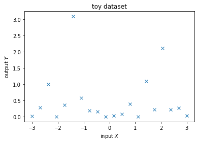
We’ll use MCMC to deal with both the kernel parameters \(\theta\) and the latent function values \(f\). Firstly, generate a data set.
[19]:
rng = np.random.RandomState(14)

X = np.linspace(-3, 3, 20)
Y = rng.exponential(np.sin(X) ** 2)

plt.figure()
plt.plot(X, Y, "x")
plt.xlabel("input $X$")
plt.ylabel("output $Y$")
plt.title("toy dataset")
plt.show()

data = (X[:, None], Y[:, None])
GPflow’s model for fully-Bayesian MCMC is called GPMC. It’s constructed like any other model, but contains a parameter V which represents the centered values of the function.
[20]:
kernel = gpflow.kernels.Matern32() + gpflow.kernels.Constant()
likelihood = gpflow.likelihoods.Exponential()
model = gpflow.models.GPMC(data, kernel, likelihood)
The V parameter already has a prior applied. We’ll add priors to the parameters also (these are rather arbitrary, for illustration).
[21]:
model.kernel.kernels[0].lengthscales.prior = tfd.Gamma(f64(1.0), f64(1.0))
model.kernel.kernels[0].variance.prior = tfd.Gamma(f64(1.0), f64(1.0))
model.kernel.kernels[1].variance.prior = tfd.Gamma(f64(1.0), f64(1.0))

gpflow.utilities.print_summary(model)
| name | class | transform | prior | trainable | shape | dtype | value |
|---|---|---|---|---|---|---|---|
| GPMC.kernel.kernels[0].variance | Parameter | Softplus | Gamma | True | () | float64 | 1.0 |
| GPMC.kernel.kernels[0].lengthscales | Parameter | Softplus | Gamma | True | () | float64 | 1.0 |
| GPMC.kernel.kernels[1].variance | Parameter | Softplus | Gamma | True | () | float64 | 1.0 |
| GPMC.V | Parameter | Identity | Normal | True | (20, 1) | float64 | [[0.... |
Running HMC is pretty similar to optimizing a model. GPflow builds on top of tensorflow_probability’s mcmc module and provides a SamplingHelper class to make interfacing easier.
We initialize HMC at the maximum a posteriori parameter values of the model.
[22]:
optimizer = gpflow.optimizers.Scipy()
maxiter = ci_niter(3000)
_ = optimizer.minimize(
    model.training_loss, model.trainable_variables, options=dict(maxiter=maxiter)
)
# We can now start HMC near maximum a posteriori (MAP)
We then run the sampler,
[23]:
num_burnin_steps = ci_niter(600)
num_samples = ci_niter(1000)

# Note that here we need model.trainable_parameters, not trainable_variables - only parameters can have priors!
hmc_helper = gpflow.optimizers.SamplingHelper(
    model.log_posterior_density, model.trainable_parameters
)

hmc = tfp.mcmc.HamiltonianMonteCarlo(
    target_log_prob_fn=hmc_helper.target_log_prob_fn, num_leapfrog_steps=10, step_size=0.01
)

adaptive_hmc = tfp.mcmc.SimpleStepSizeAdaptation(
    hmc, num_adaptation_steps=10, target_accept_prob=f64(0.75), adaptation_rate=0.1
)


@tf.function
def run_chain_fn():
    return tfp.mcmc.sample_chain(
        num_results=num_samples,
        num_burnin_steps=num_burnin_steps,
        current_state=hmc_helper.current_state,
        kernel=adaptive_hmc,
        trace_fn=lambda _, pkr: pkr.inner_results.is_accepted,
    )


samples, _ = run_chain_fn()
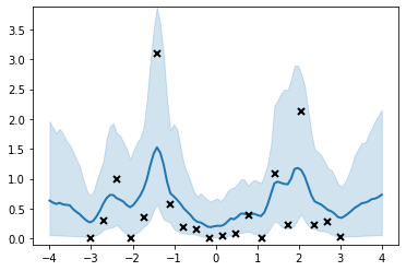
And compute the posterior prediction on a grid for plotting purposes.
[24]:
Xtest = np.linspace(-4, 4, 100)[:, None]
f_samples = []

for i in range(num_samples):
    # Note that hmc_helper.current_state contains the unconstrained variables
    for var, var_samples in zip(hmc_helper.current_state, samples):
        var.assign(var_samples[i])
    f = model.predict_f_samples(Xtest, 5)
    f_samples.append(f)
f_samples = np.vstack(f_samples)
[25]:
rate_samples = np.exp(f_samples[:, :, 0])

(line,) = plt.plot(Xtest, np.mean(rate_samples, 0), lw=2)
plt.fill_between(
    Xtest[:, 0],
    np.percentile(rate_samples, 5, axis=0),
    np.percentile(rate_samples, 95, axis=0),
    color=line.get_color(),
    alpha=0.2,
)

plt.plot(X, Y, "kx", mew=2)
_ = plt.ylim(-0.1, np.max(np.percentile(rate_samples, 95, axis=0)))
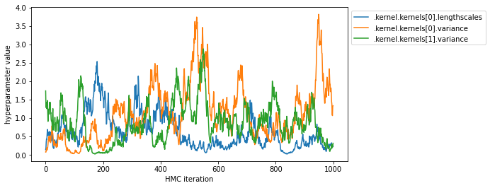
You can also display the sequence of sampled hyperparameters.
[26]:
parameter_samples = hmc_helper.convert_to_constrained_values(samples)
param_to_name = {param: name for name, param in gpflow.utilities.parameter_dict(model).items()}
name_to_index = {param_to_name[param]: i for i, param in enumerate(model.trainable_parameters)}
hyperparameters = [
    ".kernel.kernels[0].lengthscales",
    ".kernel.kernels[0].variance",
    ".kernel.kernels[1].variance",
]


plt.figure(figsize=(8, 4))
for param_name in hyperparameters:
    plt.plot(parameter_samples[name_to_index[param_name]], label=param_name)
plt.legend(bbox_to_anchor=(1.0, 1.0))
plt.xlabel("HMC iteration")
_ = plt.ylabel("hyperparameter value")
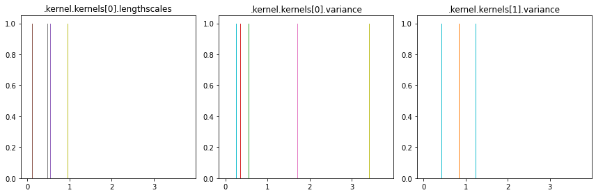
You can also inspect the marginal of the posterior samples.
[27]:
fig, axes = plt.subplots(1, len(hyperparameters), sharex=True, figsize=(12, 4))
for ax, param_name in zip(axes, hyperparameters):
    ax.hist(parameter_samples[name_to_index[param_name]], bins=20)
    ax.set_title(param_name)
plt.tight_layout()
Prior on constrained and unconstrained parameters
GPflow’s Parameter class provides options for setting a prior. Parameter wraps a constrained tensor and provides computation of the gradient with respect to unconstrained transformation of that tensor. The user can set a prior either in constrained space or unconstrained space.
By default, the prior for the Parameter is set on the constrained space. To explicitly set the space on which the prior is defined, use the prior_on keyword argument:
[28]:
prior_distribution = tfd.Normal(f64(0.0), f64(1.0))
_ = gpflow.Parameter(1.0, prior_on="unconstrained", prior=prior_distribution)
_ = gpflow.Parameter(1.0, prior_on="constrained", prior=prior_distribution)
gpflow.optimizers.SamplingHelper makes sure that the prior density correctly reflects the space in which the prior is defined.
Below we repeat the same experiment as before, but with some priors defined in the unconstrained space. We are using the exponential transform to ensure positivity of the kernel parameters (set_default_positive_bijector("exp")), so a log-normal prior on a constrained parameter corresponds to a normal prior on the unconstrained space:
[29]:
gpflow.config.set_default_positive_bijector("exp")
gpflow.config.set_default_positive_minimum(1e-6)

rng = np.random.RandomState(42)
data = synthetic_data(30, rng)

kernel = gpflow.kernels.Matern52(lengthscales=0.3)
meanf = gpflow.mean_functions.Linear(1.0, 0.0)
model = gpflow.models.GPR(data, kernel, meanf)
model.likelihood.variance.assign(0.01)

mu = f64(0.0)
std = f64(4.0)
one = f64(1.0)

model.kernel.lengthscales.prior_on = "unconstrained"
model.kernel.lengthscales.prior = tfd.Normal(mu, std)
model.kernel.variance.prior_on = "unconstrained"
model.kernel.variance.prior = tfd.Normal(mu, std)
model.likelihood.variance.prior_on = "unconstrained"
model.likelihood.variance.prior = tfd.Normal(mu, std)

model.mean_function.A.prior_on = "constrained"
model.mean_function.A.prior = tfd.Normal(mu, std)
model.mean_function.b.prior_on = "constrained"
model.mean_function.b.prior = tfd.Normal(mu, std)

model.kernel.lengthscales.prior_on
[29]:
<PriorOn.UNCONSTRAINED: 'unconstrained'>
Let’s run HMC and plot chain traces:
[30]:
num_burnin_steps = ci_niter(300)
num_samples = ci_niter(500)

hmc_helper = gpflow.optimizers.SamplingHelper(
    model.log_posterior_density, model.trainable_parameters
)

hmc = tfp.mcmc.HamiltonianMonteCarlo(
    target_log_prob_fn=hmc_helper.target_log_prob_fn, num_leapfrog_steps=10, step_size=0.01
)
adaptive_hmc = tfp.mcmc.SimpleStepSizeAdaptation(
    hmc, num_adaptation_steps=10, target_accept_prob=f64(0.75), adaptation_rate=0.1
)


@tf.function
def run_chain_fn_unconstrained():
    return tfp.mcmc.sample_chain(
        num_results=num_samples,
        num_burnin_steps=num_burnin_steps,
        current_state=hmc_helper.current_state,
        kernel=adaptive_hmc,
        trace_fn=lambda _, pkr: pkr.inner_results.is_accepted,
    )


samples, traces = run_chain_fn_unconstrained()
parameter_samples = hmc_helper.convert_to_constrained_values(samples)

param_to_name = {param: name for name, param in gpflow.utilities.parameter_dict(model).items()}
marginal_samples(samples, model.trainable_parameters, "unconstrained variable samples")
marginal_samples(parameter_samples, model.trainable_parameters, "constrained parameter samples")