Basic (Gaussian likelihood) GP regression model

This notebook shows the different steps for creating and using a standard GP regression model, including: - reading and formatting data - choosing a kernel function - choosing a mean function (optional) - creating the model - viewing, getting, and setting model parameters - optimizing the model parameters - making predictions

We focus here on the implementation of the models in GPflow; for more intuition on these models, see A Practical Guide to Gaussian Processes and A Visual Exploration of Gaussian Processes.

import gpflow
import numpy as np
import matplotlib.pyplot as plt
import tensorflow as tf
from gpflow.utilities import print_summary

# The lines below are specific to the notebook format
%matplotlib inline
plt.rcParams["figure.figsize"] = (12, 6)

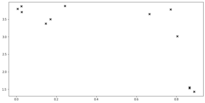
X and Y denote the input and output values. NOTE: X and Y must be two-dimensional NumPy arrays, \(N \times 1\) or \(N \times D\), where \(D\) is the number of input dimensions/features, with the same number of rows as \(N\) (one for each data point):

data = np.genfromtxt("data/regression_1D.csv", delimiter=",")
X = data[:, 0].reshape(-1, 1)
Y = data[:, 1].reshape(-1, 1)

_ = plt.plot(X, Y, "kx", mew=2)

We will consider the following probabilistic model:

\begin{equation} Y_i = f(X_i) + \varepsilon_i\,, \end{equation}

where \(f \sim \mathcal{GP}(\mu(\cdot), k(\cdot, \cdot'))\), and \(\varepsilon \sim \mathcal{N}(0, \tau^2 I)\).

Choose a kernel

Several kernels (covariance functions) are implemented in GPflow. You can easily combine them to create new ones (see Manipulating kernels). You can also implement new covariance functions, as shown in the Kernel design notebook. Here, we will use a simple one:

k = gpflow.kernels.Matern52()

2022-03-18 10:10:33.383692: I tensorflow/stream_executor/cuda/cuda_gpu_executor.cc:936] successful NUMA node read from SysFS had negative value (-1), but there must be at least one NUMA node, so returning NUMA node zero
2022-03-18 10:10:33.386689: W tensorflow/stream_executor/platform/default/dso_loader.cc:64] Could not load dynamic library 'libcusolver.so.11'; dlerror: libcusolver.so.11: cannot open shared object file: No such file or directory
2022-03-18 10:10:33.387110: W tensorflow/core/common_runtime/gpu/gpu_device.cc:1850] Cannot dlopen some GPU libraries. Please make sure the missing libraries mentioned above are installed properly if you would like to use GPU. Follow the guide at https://www.tensorflow.org/install/gpu for how to download and setup the required libraries for your platform.
Skipping registering GPU devices...
2022-03-18 10:10:33.388004: I tensorflow/core/platform/cpu_feature_guard.cc:151] This TensorFlow binary is optimized with oneAPI Deep Neural Network Library (oneDNN) to use the following CPU instructions in performance-critical operations:  AVX2 FMA
To enable them in other operations, rebuild TensorFlow with the appropriate compiler flags.

For more advanced kernels see the advanced kernel notebook (including kernels defined on subspaces). A summary of the kernel can be obtained by

print_summary(k)

╒═══════════════════════╤═══════════╤═════════════╤═════════╤═════════════╤═════════╤═════════╤═════════╕
│ name                  │ class     │ transform   │ prior   │ trainable   │ shape   │ dtype   │   value │
╞═══════════════════════╪═══════════╪═════════════╪═════════╪═════════════╪═════════╪═════════╪═════════╡
│ Matern52.variance     │ Parameter │ Softplus    │         │ True        │ ()      │ float64 │       1 │
├───────────────────────┼───────────┼─────────────┼─────────┼─────────────┼─────────┼─────────┼─────────┤
│ Matern52.lengthscales │ Parameter │ Softplus    │         │ True        │ ()      │ float64 │       1 │
╘═══════════════════════╧═══════════╧═════════════╧═════════╧═════════════╧═════════╧═════════╧═════════╛

The Matern 5/2 kernel has two parameters: lengthscales, which encodes the “wiggliness” of the GP, and variance, which tunes the amplitude. They are both set to 1.0 as the default value. For more details on the meaning of the other columns, see Manipulating kernels.

Choose a mean function (optional)

It is common to choose \(\mu = 0\), which is the GPflow default.

However, if there is a clear pattern (such as a mean value of Y that is far away from 0, or a linear trend in the data), mean functions can be beneficial. Some simple ones are provided in the gpflow.mean_functions module.

Here’s how to define a linear mean function:

meanf = gpflow.mean_functions.Linear()

Construct a model

A GPflow model is created by instantiating one of the GPflow model classes, in this case GPR. We’ll make a kernel k and instantiate a GPR object using the generated data and the kernel. We’ll also set the variance of the likelihood to a sensible initial guess.

m = gpflow.models.GPR(data=(X, Y), kernel=k, mean_function=None)

A summary of the model can be obtained by

print_summary(m)

╒═════════════════════════╤═══════════╤══════════════════╤═════════╤═════════════╤═════════╤═════════╤═════════╕
│ name                    │ class     │ transform        │ prior   │ trainable   │ shape   │ dtype   │   value │
╞═════════════════════════╪═══════════╪══════════════════╪═════════╪═════════════╪═════════╪═════════╪═════════╡
│ GPR.kernel.variance     │ Parameter │ Softplus         │         │ True        │ ()      │ float64 │       1 │
├─────────────────────────┼───────────┼──────────────────┼─────────┼─────────────┼─────────┼─────────┼─────────┤
│ GPR.kernel.lengthscales │ Parameter │ Softplus         │         │ True        │ ()      │ float64 │       1 │
├─────────────────────────┼───────────┼──────────────────┼─────────┼─────────────┼─────────┼─────────┼─────────┤
│ GPR.likelihood.variance │ Parameter │ Softplus + Shift │         │ True        │ ()      │ float64 │       1 │
╘═════════════════════════╧═══════════╧══════════════════╧═════════╧═════════════╧═════════╧═════════╧═════════╛

The first two lines correspond to the kernel parameters, and the third one gives the likelihood parameter (the noise variance \(\tau^2\) in our model).

You can access those values and manually set them to sensible initial guesses. For example:

m.likelihood.variance.assign(0.01)
m.kernel.lengthscales.assign(0.3)

<tf.Variable 'UnreadVariable' shape=() dtype=float64, numpy=-1.0502256128148466>

Optimize the model parameters

To obtain meaningful predictions, you need to tune the model parameters (that is, the parameters of the kernel, the likelihood, and the mean function if applicable) to the data at hand.

There are several optimizers available in GPflow. Here we use the Scipy optimizer, which by default implements the L-BFGS-B algorithm. (You can select other algorithms by using the method= keyword argument to its minimize method; see the SciPy documentation for details of available options.)

opt = gpflow.optimizers.Scipy()

In order to train the model, we need to maximize the log marginal likelihood. GPflow models define a training_loss that can be passed to the minimize method of an optimizer; in this case it is simply the negative log marginal likelihood. We also need to specify the variables to train with m.trainable_variables, and the number of iterations.

opt_logs = opt.minimize(m.training_loss, m.trainable_variables, options=dict(maxiter=100))
print_summary(m)

2022-03-18 10:10:33.512016: W tensorflow/python/util/util.cc:368] Sets are not currently considered sequences, but this may change in the future, so consider avoiding using them.

╒═════════════════════════╤═══════════╤══════════════════╤═════════╤═════════════╤═════════╤═════════╤═══════════╕
│ name                    │ class     │ transform        │ prior   │ trainable   │ shape   │ dtype   │     value │
╞═════════════════════════╪═══════════╪══════════════════╪═════════╪═════════════╪═════════╪═════════╪═══════════╡
│ GPR.kernel.variance     │ Parameter │ Softplus         │         │ True        │ ()      │ float64 │ 7.96581   │
├─────────────────────────┼───────────┼──────────────────┼─────────┼─────────────┼─────────┼─────────┼───────────┤
│ GPR.kernel.lengthscales │ Parameter │ Softplus         │         │ True        │ ()      │ float64 │ 0.212416  │
├─────────────────────────┼───────────┼──────────────────┼─────────┼─────────────┼─────────┼─────────┼───────────┤
│ GPR.likelihood.variance │ Parameter │ Softplus + Shift │         │ True        │ ()      │ float64 │ 0.0057594 │
╘═════════════════════════╧═══════════╧══════════════════╧═════════╧═════════════╧═════════╧═════════╧═══════════╛

Notice how the value column has changed.

The local optimum found by Maximum Likelihood might not be the one you want (for example, it might be overfitting or oversmooth). This depends on the initial values of the hyperparameters, and is specific to each dataset. As an alternative to Maximum Likelihood, Markov Chain Monte Carlo (MCMC) is also available.

Make predictions

We can now use the model to make some predictions at the new points Xnew. You might be interested in predicting two different quantities: the latent function values f(Xnew) (the denoised signal), or the values of new observations y(Xnew) (signal + noise). Because we are dealing with Gaussian probabilistic models, the predictions typically produce a mean and variance as output. Alternatively, you can obtain samples of f(Xnew) or the log density of the new data points (Xnew, Ynew).

GPflow models have several prediction methods:

• m.predict_f returns the mean and marginal variance of \(f\) at the points Xnew.

• m.predict_f with argument full_cov=True returns the mean and the full covariance matrix of \(f\) at the points Xnew.

• m.predict_f_samples returns samples of the latent function.

• m.predict_y returns the mean and variance of a new data point (that is, it includes the noise variance).

• m.predict_log_density returns the log density of the observations Ynew at Xnew.

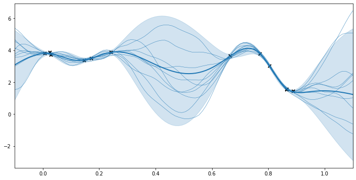
We use predict_f and predict_f_samples to plot 95% confidence intervals and samples from the posterior distribution.

## generate test points for prediction
xx = np.linspace(-0.1, 1.1, 100).reshape(100, 1)  # test points must be of shape (N, D)

## predict mean and variance of latent GP at test points
mean, var = m.predict_f(xx)

## generate 10 samples from posterior
tf.random.set_seed(1)  # for reproducibility
samples = m.predict_f_samples(xx, 10)  # shape (10, 100, 1)

## plot
plt.figure(figsize=(12, 6))
plt.plot(X, Y, "kx", mew=2)
plt.plot(xx, mean, "C0", lw=2)
plt.fill_between(
    xx[:, 0],
    mean[:, 0] - 1.96 * np.sqrt(var[:, 0]),
    mean[:, 0] + 1.96 * np.sqrt(var[:, 0]),
    color="C0",
    alpha=0.2,
)

plt.plot(xx, samples[:, :, 0].numpy().T, "C0", linewidth=0.5)
_ = plt.xlim(-0.1, 1.1)

GP regression in higher dimensions

Very little changes when the input space has more than one dimension. By default, the lengthscales is an isotropic (scalar) parameter. It is generally recommended that you allow to tune a different lengthscale for each dimension (Automatic Relevance Determination, ARD): simply initialize lengthscales with an array of length \(D\) corresponding to the input dimension of X. See Manipulating kernels for further information.

Further reading

• Stochastic Variational Inference for scalability with SVGP for cases where there are a large number of observations.

• Ordinal regression if the data is ordinal.

• Multi-output models and coregionalisation if Y is multidimensional.