Manipulating GPflow models

One of the key ingredients in GPflow is the model class, which enables you to carefully control parameters. This notebook shows how some of these parameter control features work, and how to build your own model with GPflow. First we’ll look at:

• how to view models and parameters

• how to set parameter values

• how to constrain parameters (for example, variance > 0)

• how to fix model parameters

• how to apply priors to parameters

• how to optimize models

Then we’ll show how to build a simple logistic regression model, demonstrating the ease of the parameter framework.

GPy users should feel right at home, but there are some small differences.

First, let’s deal with the usual notebook boilerplate and make a simple GP regression model. See Basic (Gaussian likelihood) GP regression model for specifics of the model; we just want some parameters to play with.

import numpy as np
import gpflow
import tensorflow_probability as tfp
from gpflow.utilities import print_summary, set_trainable, to_default_float

We begin by creating a very simple GP regression model:

# generate toy data
np.random.seed(1)
X = np.random.rand(20, 1)
Y = np.sin(12 * X) + 0.66 * np.cos(25 * X) + np.random.randn(20, 1) * 0.01

m = gpflow.models.GPR((X, Y), kernel=gpflow.kernels.Matern32() + gpflow.kernels.Linear())

2022-03-18 10:17:42.151960: I tensorflow/stream_executor/cuda/cuda_gpu_executor.cc:936] successful NUMA node read from SysFS had negative value (-1), but there must be at least one NUMA node, so returning NUMA node zero
2022-03-18 10:17:42.155313: W tensorflow/stream_executor/platform/default/dso_loader.cc:64] Could not load dynamic library 'libcusolver.so.11'; dlerror: libcusolver.so.11: cannot open shared object file: No such file or directory
2022-03-18 10:17:42.155809: W tensorflow/core/common_runtime/gpu/gpu_device.cc:1850] Cannot dlopen some GPU libraries. Please make sure the missing libraries mentioned above are installed properly if you would like to use GPU. Follow the guide at https://www.tensorflow.org/install/gpu for how to download and setup the required libraries for your platform.
Skipping registering GPU devices...
2022-03-18 10:17:42.156441: I tensorflow/core/platform/cpu_feature_guard.cc:151] This TensorFlow binary is optimized with oneAPI Deep Neural Network Library (oneDNN) to use the following CPU instructions in performance-critical operations:  AVX2 FMA
To enable them in other operations, rebuild TensorFlow with the appropriate compiler flags.

Viewing, getting, and setting parameters

You can display the state of the model in a terminal by using print_summary(m). You can change the display format using the fmt keyword argument, e.g. 'html'. In a notebook, you can also use fmt='notebook' or set the default printing format as notebook:

print_summary(m, fmt="notebook")

name	class	transform	prior	trainable	shape	dtype	value
GPR.kernel.kernels[0].variance	Parameter	Softplus		True	()	float64	1
GPR.kernel.kernels[0].lengthscales	Parameter	Softplus		True	()	float64	1
GPR.kernel.kernels[1].variance	Parameter	Softplus		True	()	float64	1
GPR.likelihood.variance	Parameter	Softplus + Shift		True	()	float64	1

gpflow.config.set_default_summary_fmt("notebook")

This model has four parameters. The kernel is made of the sum of two parts. The first (counting from zero) is a Matern32 kernel that has a variance parameter and a lengthscales parameter; the second is a linear kernel that has only a variance parameter. There is also a parameter that controls the variance of the noise, as part of the likelihood.

All the model variables have been initialized at 1.0. You can access individual parameters in the same way that you display the state of the model in a terminal; for example, to see all the parameters that are part of the likelihood, run:

print_summary(m.likelihood)

name	class	transform	prior	trainable	shape	dtype	value
Gaussian.variance	Parameter	Softplus + Shift		True	()	float64	1

This gets more useful with more complex models!

To set the value of a parameter, just use assign():

m.kernel.kernels[0].lengthscales.assign(0.5)
m.likelihood.variance.assign(0.01)
print_summary(m, fmt="notebook")

name	class	transform	prior	trainable	shape	dtype	value
GPR.kernel.kernels[0].variance	Parameter	Softplus		True	()	float64	1
GPR.kernel.kernels[0].lengthscales	Parameter	Softplus		True	()	float64	0.5
GPR.kernel.kernels[1].variance	Parameter	Softplus		True	()	float64	1
GPR.likelihood.variance	Parameter	Softplus + Shift		True	()	float64	0.01

Constraints and trainable variables

GPflow helpfully creates an unconstrained representation of all the variables. In the previous example, all the variables are constrained positively (see the transform column in the table); the unconstrained representation is given by \(\alpha = \log(\exp(\theta)-1)\). The trainable_parameters property returns the constrained values:

m.trainable_parameters

2022-03-18 10:17:42.213893: W tensorflow/python/util/util.cc:368] Sets are not currently considered sequences, but this may change in the future, so consider avoiding using them.

(<Parameter: name=softplus, dtype=float64, shape=[], fn="softplus", numpy=0.5>,
 <Parameter: name=softplus, dtype=float64, shape=[], fn="softplus", numpy=1.0>,
 <Parameter: name=softplus, dtype=float64, shape=[], fn="softplus", numpy=1.0>,
 <Parameter: name=chain_of_shift_of_softplus, dtype=float64, shape=[], fn="chain_of_shift_of_softplus", numpy=0.009999999999999998>)

Each parameter has an unconstrained_variable attribute that enables you to access the unconstrained value as a TensorFlow Variable.

p = m.kernel.kernels[0].lengthscales
p.unconstrained_variable

<tf.Variable 'Variable:0' shape=() dtype=float64, numpy=-0.43275212956718856>

You can also check the unconstrained value as follows:

p.transform.inverse(p)

<tf.Tensor: shape=(), dtype=float64, numpy=-0.43275212956718856>

Constraints are handled by the Bijector classes from the tensorflow_probability package. You might prefer to use the constraint \(\alpha = \log(\theta)\); this is easily done by replacing the parameter with one that has a different transform attribute (here we make sure to copy all other attributes across from the old parameter; this is not necessary when there is no prior and the trainable state is still the default of True):

old_parameter = m.kernel.kernels[0].lengthscales
new_parameter = gpflow.Parameter(
    old_parameter,
    trainable=old_parameter.trainable,
    prior=old_parameter.prior,
    name=old_parameter.name.split(":")[0],  # tensorflow is weird and adds ':0' to the name
    transform=tfp.bijectors.Exp(),
)
m.kernel.kernels[0].lengthscales = new_parameter

Though the lengthscale itself remains the same, the unconstrained lengthscale has changed:

p.transform.inverse(p)

<tf.Tensor: shape=(), dtype=float64, numpy=-0.43275212956718856>

To replace the transform of a parameter you need to recreate the parameter with updated transform:

p = m.kernel.kernels[0].variance
m.kernel.kernels[0].variance = gpflow.Parameter(p.numpy(), transform=tfp.bijectors.Exp())

print_summary(m, fmt="notebook")

name	class	transform	prior	trainable	shape	dtype	value
GPR.kernel.kernels[0].variance	Parameter	Exp		True	()	float64	1
GPR.kernel.kernels[0].lengthscales	Parameter	Exp		True	()	float64	0.5
GPR.kernel.kernels[1].variance	Parameter	Softplus		True	()	float64	1
GPR.likelihood.variance	Parameter	Softplus + Shift		True	()	float64	0.01

Changing whether a parameter will be trained in optimization

Another helpful feature is the ability to fix parameters. To do this, simply set the trainable attribute to False; this is shown in the trainable column of the representation, and the corresponding variable is removed from the free state.

set_trainable(m.kernel.kernels[1].variance, False)
print_summary(m)

name	class	transform	prior	trainable	shape	dtype	value
GPR.kernel.kernels[0].variance	Parameter	Exp		True	()	float64	1
GPR.kernel.kernels[0].lengthscales	Parameter	Exp		True	()	float64	0.5
GPR.kernel.kernels[1].variance	Parameter	Softplus		False	()	float64	1
GPR.likelihood.variance	Parameter	Softplus + Shift		True	()	float64	0.01

m.trainable_parameters

(<Parameter: name=softplus, dtype=float64, shape=[], fn="exp", numpy=0.5>,
 <Parameter: name=exp, dtype=float64, shape=[], fn="exp", numpy=1.0>,
 <Parameter: name=chain_of_shift_of_softplus, dtype=float64, shape=[], fn="chain_of_shift_of_softplus", numpy=0.009999999999999998>)

To unfix a parameter, just set the trainable attribute to True again.

set_trainable(m.kernel.kernels[1].variance, True)
print_summary(m)

name	class	transform	prior	trainable	shape	dtype	value
GPR.kernel.kernels[0].variance	Parameter	Exp		True	()	float64	1
GPR.kernel.kernels[0].lengthscales	Parameter	Exp		True	()	float64	0.5
GPR.kernel.kernels[1].variance	Parameter	Softplus		True	()	float64	1
GPR.likelihood.variance	Parameter	Softplus + Shift		True	()	float64	0.01

NOTE: If you want to recursively change the trainable status of an object that contains parameters, you must use the set_trainable() utility function.

A module (e.g. a model, kernel, likelihood, … instance) does not have a trainable attribute:

try:
    m.kernel.trainable
except AttributeError:
    print(f"{m.kernel.__class__.__name__} does not have a trainable attribute")

Sum does not have a trainable attribute

set_trainable(m.kernel, False)
print_summary(m)

name	class	transform	prior	trainable	shape	dtype	value
GPR.kernel.kernels[0].variance	Parameter	Exp		False	()	float64	1
GPR.kernel.kernels[0].lengthscales	Parameter	Exp		False	()	float64	0.5
GPR.kernel.kernels[1].variance	Parameter	Softplus		False	()	float64	1
GPR.likelihood.variance	Parameter	Softplus + Shift		True	()	float64	0.01

Priors

You can set priors in the same way as transforms and trainability, by using tensorflow_probability distribution objects. Let’s set a Gamma prior on the variance of the Matern32 kernel.

k = gpflow.kernels.Matern32()
k.variance.prior = tfp.distributions.Gamma(to_default_float(2), to_default_float(3))

print_summary(k)

name	class	transform	prior	trainable	shape	dtype	value
Matern32.variance	Parameter	Softplus	Gamma	True	()	float64	1
Matern32.lengthscales	Parameter	Softplus		True	()	float64	1

m.kernel.kernels[0].variance.prior = tfp.distributions.Gamma(
    to_default_float(2), to_default_float(3)
)
print_summary(m)

name	class	transform	prior	trainable	shape	dtype	value
GPR.kernel.kernels[0].variance	Parameter	Exp	Gamma	False	()	float64	1
GPR.kernel.kernels[0].lengthscales	Parameter	Exp		False	()	float64	0.5
GPR.kernel.kernels[1].variance	Parameter	Softplus		False	()	float64	1
GPR.likelihood.variance	Parameter	Softplus + Shift		True	()	float64	0.01

Optimization

To optimize your model, first create an instance of an optimizer (in this case, gpflow.optimizers.Scipy), which has optional arguments that are passed to scipy.optimize.minimize (we minimize the negative log likelihood). Then, call the minimize method of that optimizer, with your model as the optimization target. Variables that have priors are maximum a priori (MAP) estimated, that is, we add the log prior to the log likelihood, and otherwise use Maximum Likelihood.

opt = gpflow.optimizers.Scipy()
opt.minimize(m.training_loss, variables=m.trainable_variables)

      fun: 27.18433901409803
 hess_inv: <1x1 LbfgsInvHessProduct with dtype=float64>
      jac: array([-1.02640285e-06])
  message: 'CONVERGENCE: NORM_OF_PROJECTED_GRADIENT_<=_PGTOL'
     nfev: 8
      nit: 7
     njev: 8
   status: 0
  success: True
        x: array([-0.36990459])

Building new models

To build new models, you’ll need to inherit from gpflow.models.BayesianModel. Parameters are instantiated with gpflow.Parameter. You might also be interested in gpflow.Module (a subclass of tf.Module), which acts as a ‘container’ for Parameters (for example, kernels are gpflow.Modules).

In this very simple demo, we’ll implement linear multiclass classification.

There are two parameters: a weight matrix and a bias (offset). You can use Parameter objects directly, like any TensorFlow tensor.

The training objective depends on the type of model; it may be possible to implement the exact (log)marginal likelihood, or only a lower bound to the log marginal likelihood (ELBO). You need to implement this as the maximum_log_likelihood_objective method. The BayesianModel parent class provides a log_posterior_density method that returns the maximum_log_likelihood_objective plus the sum of the log-density of any priors on hyperparameters, which can be used for MCMC. GPflow provides mixin classes that define a training_loss method that returns the negative of (maximum likelihood objective + log prior density) for MLE/MAP estimation to be passed to optimizer’s minimize method. Models that derive from InternalDataTrainingLossMixin are expected to store the data internally, and their training_loss does not take any arguments and can be passed directly to minimize. Models that take data as an argument to their maximum_log_likelihood_objective method derive from ExternalDataTrainingLossMixin, which provides a training_loss_closure to take the data and return the appropriate closure for optimizer.minimize. This is also discussed in the GPflow with TensorFlow 2 notebook.

import tensorflow as tf


class LinearMulticlass(gpflow.models.BayesianModel, gpflow.models.InternalDataTrainingLossMixin):
    # The InternalDataTrainingLossMixin provides the training_loss method.
    # (There is also an ExternalDataTrainingLossMixin for models that do not encapsulate data.)

    def __init__(self, X, Y, name=None):
        super().__init__(name=name)  # always call the parent constructor

        self.X = X.copy()  # X is a NumPy array of inputs
        self.Y = Y.copy()  # Y is a 1-of-k (one-hot) representation of the labels

        self.num_data, self.input_dim = X.shape
        _, self.num_classes = Y.shape

        # make some parameters
        self.W = gpflow.Parameter(np.random.randn(self.input_dim, self.num_classes))
        self.b = gpflow.Parameter(np.random.randn(self.num_classes))

        # ^^ You must make the parameters attributes of the class for
        # them to be picked up by the model. i.e. this won't work:
        #
        # W = gpflow.Parameter(...    <-- must be self.W

    def maximum_log_likelihood_objective(self):
        p = tf.nn.softmax(
            tf.matmul(self.X, self.W) + self.b
        )  # Parameters can be used like a tf.Tensor
        return tf.reduce_sum(tf.math.log(p) * self.Y)  # be sure to return a scalar

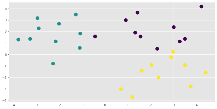
…and that’s it. Let’s build a really simple demo to show that it works.

np.random.seed(123)
X = np.vstack(
    [
        np.random.randn(10, 2) + [2, 2],
        np.random.randn(10, 2) + [-2, 2],
        np.random.randn(10, 2) + [2, -2],
    ]
)
Y = np.repeat(np.eye(3), 10, 0)

import matplotlib.pyplot as plt

plt.style.use("ggplot")
%matplotlib inline

plt.rcParams["figure.figsize"] = (12, 6)
_ = plt.scatter(X[:, 0], X[:, 1], 100, np.argmax(Y, 1), lw=2, cmap=plt.cm.viridis)

m = LinearMulticlass(X, Y)
m

<__main__.LinearMulticlass object at 0x7feab298bd90>

name	class	transform	prior	trainable	shape	dtype	value
LinearMulticlass.W	Parameter	Identity		True	(2, 3)	float64	[[-0.77270871, 0.79486267, 0.31427199...
LinearMulticlass.b	Parameter	Identity		True	(3,)	float64	[ 0.04549008 -0.23309206 -1.19830114]

opt = gpflow.optimizers.Scipy()
opt.minimize(m.training_loss, variables=m.trainable_variables)

      fun: 1.2560984620980772e-05
 hess_inv: <9x9 LbfgsInvHessProduct with dtype=float64>
      jac: array([ 4.28392990e-06,  1.15665823e-06, -5.44058813e-06, -2.77570188e-06,
        2.97110223e-06, -1.95400347e-07, -8.81900274e-07,  2.52856126e-06,
       -1.64666099e-06])
  message: 'CONVERGENCE: NORM_OF_PROJECTED_GRADIENT_<=_PGTOL'
     nfev: 27
      nit: 26
     njev: 27
   status: 0
  success: True
        x: array([  8.55849743, -30.63655328,  22.4144818 ,  23.79332963,
        21.27896803, -44.17402754,  11.85784428, -12.94743432,
        -0.29631308])

xx, yy = np.mgrid[-4:4:200j, -4:4:200j]
X_test = np.vstack([xx.flatten(), yy.flatten()]).T
f_test = np.dot(X_test, m.W.numpy()) + m.b.numpy()
p_test = np.exp(f_test)
p_test /= p_test.sum(1)[:, None]

plt.figure(figsize=(12, 6))
for i in range(3):
    plt.contour(xx, yy, p_test[:, i].reshape(200, 200), [0.5], colors="k", linewidths=1)
_ = plt.scatter(X[:, 0], X[:, 1], 100, np.argmax(Y, 1), lw=2, cmap=plt.cm.viridis)

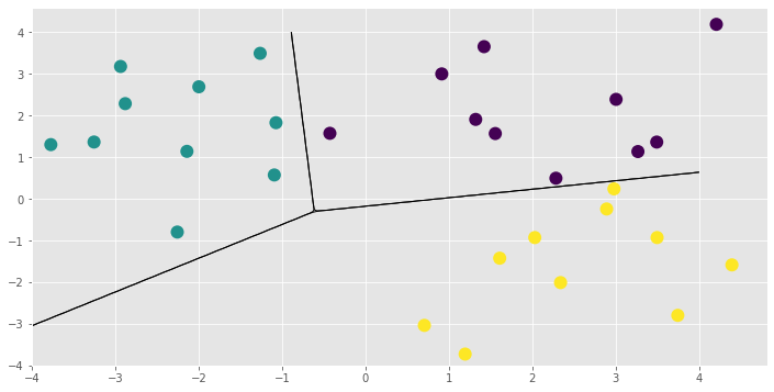
That concludes the new model example and this notebook. You might want to see for yourself that the LinearMulticlass model and its parameters have all the functionality demonstrated here. You could also add some priors and run Hamiltonian Monte Carlo using the HMC optimizer gpflow.train.HMC and its sample method. See Markov Chain Monte Carlo (MCMC) for more information on running the sampler.