Gaussian process regression with varying output noise

This notebook shows how to construct a Gaussian process model where different noise is assumed for different data points. The model is:

\begin{align} f(\cdot) &\sim \mathcal{GP}\big(0, k(\cdot, \cdot)\big) \\ y_i | f, x_i &\sim \mathcal N\big(y_i; f(x_i), \sigma^2_i\big) \end{align}

We’ll demonstrate two methods. In the first demonstration, we’ll assume that the noise variance is known for every data point. We’ll incorporate the known noise variances \(\sigma^2_i\) into the data matrix \(\mathbf Y\), make a likelihood that can deal with this structure, and implement inference using variational GPs with natural gradients.

In the second demonstration, we’ll assume that the noise variance is not known, but we’d like to estimate it for different groups of data. We’ll show how to construct an appropriate likelihood for this task and set up inference similarly to the first demonstration, with optimization over the noise variances.

import numpy as np
import tensorflow as tf
import gpflow
from gpflow.ci_utils import ci_niter
from gpflow.optimizers import NaturalGradient
from gpflow import set_trainable
import matplotlib.pyplot as plt

%matplotlib inline

Demo 1: known noise variances

Generate synthetic data

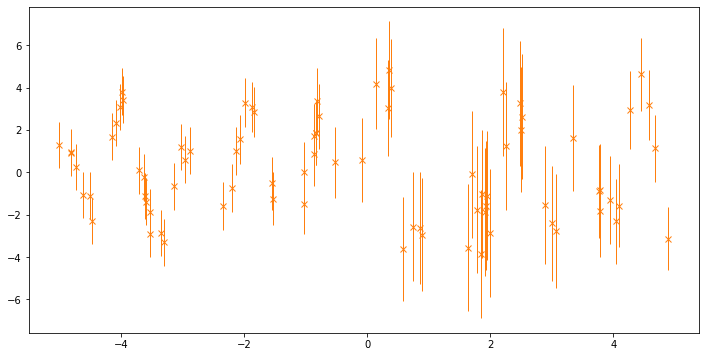
We create a utility function to generate synthetic data, including noise that varies amongst the data:

np.random.seed(1)  # for reproducibility


def generate_data(N=80):
    X = np.random.rand(N)[:, None] * 10 - 5  # Inputs, shape N x 1
    F = 2.5 * np.sin(6 * X) + np.cos(3 * X)  # Mean function values
    NoiseVar = 2 * np.exp(-((X - 2) ** 2) / 4) + 0.3  # Noise variances
    Y = F + np.random.randn(N, 1) * np.sqrt(NoiseVar)  # Noisy data
    return X, Y, NoiseVar


X, Y, NoiseVar = generate_data()

Here’s a plot of the data, with error bars representing two standard deviations:

fig, ax = plt.subplots(1, 1, figsize=(12, 6))
_ = ax.errorbar(
    X.squeeze(),
    Y.squeeze(),
    yerr=2 * (np.sqrt(NoiseVar)).squeeze(),
    marker="x",
    lw=0,
    elinewidth=1.0,
    color="C1",
)

Make a Y matrix that includes the variances

We need to tell the GP model what the variance is for each data point. To do this, we’ll concatenate the observations with the variances into a single data matrix:

Y_data = np.hstack([Y, NoiseVar])

Make a new likelihood

To cope with this data structure, we’ll build a new likelihood. Note how the code extracts the observations Y and the variances NoiseVar from the data. For more information on creating new likelihoods, see Likelihood design. Here, we’re implementing the log_prob function (which computes the log-probability of the data given the latent function) and variational_expectations, which computes the expected log-probability under a Gaussian distribution on the function, and is needed in the evaluation of the evidence lower bound (ELBO). Check out the docstring for the Likelihood object for more information on what these functions do.

class HeteroskedasticGaussian(gpflow.likelihoods.Likelihood):
    def __init__(self, **kwargs):
        # this likelihood expects a single latent function F, and two columns in the data matrix Y:
        super().__init__(latent_dim=1, observation_dim=2, **kwargs)

    def _log_prob(self, F, Y):
        # log_prob is used by the quadrature fallback of variational_expectations and predict_log_density.
        # Because variational_expectations is implemented analytically below, this is not actually needed,
        # but is included for pedagogical purposes.
        # Note that currently relying on the quadrature would fail due to https://github.com/GPflow/GPflow/issues/966
        Y, NoiseVar = Y[:, 0], Y[:, 1]
        return gpflow.logdensities.gaussian(Y, F, NoiseVar)

    def _variational_expectations(self, Fmu, Fvar, Y):
        Y, NoiseVar = Y[:, 0], Y[:, 1]
        Fmu, Fvar = Fmu[:, 0], Fvar[:, 0]
        return (
            -0.5 * np.log(2 * np.pi)
            - 0.5 * tf.math.log(NoiseVar)
            - 0.5 * (tf.math.square(Y - Fmu) + Fvar) / NoiseVar
        )

    # The following two methods are abstract in the base class.
    # They need to be implemented even if not used.

    def _predict_log_density(self, Fmu, Fvar, Y):
        raise NotImplementedError

    def _predict_mean_and_var(self, Fmu, Fvar):
        raise NotImplementedError

Put it together with Variational Gaussian Process (VGP)

Here we’ll build a variational GP model with the previous likelihood on the dataset that we generated. We’ll use the natural gradient optimizer (see Natural gradients for more information).

The variational GP object is capable of variational inference with any GPflow-derived likelihood. Usually, the inference is an inexact (but pretty good) approximation, but in the special case considered here, where the noise is Gaussian, it will achieve exact inference. Optimizing over the variational parameters is easy using the natural gradients method, which provably converges in a single step.

Note: We mark the variational parameters as not trainable so that they are not included in the model.trainable_variables when we optimize using the Adam optimizer. We train the variational parameters separately using the natural gradient method.

# model construction
likelihood = HeteroskedasticGaussian()
kernel = gpflow.kernels.Matern52(lengthscales=0.5)
model = gpflow.models.VGP((X, Y_data), kernel=kernel, likelihood=likelihood, num_latent_gps=1)

2022-03-18 10:03:55.556416: I tensorflow/stream_executor/cuda/cuda_gpu_executor.cc:936] successful NUMA node read from SysFS had negative value (-1), but there must be at least one NUMA node, so returning NUMA node zero
2022-03-18 10:03:55.559838: W tensorflow/stream_executor/platform/default/dso_loader.cc:64] Could not load dynamic library 'libcusolver.so.11'; dlerror: libcusolver.so.11: cannot open shared object file: No such file or directory
2022-03-18 10:03:55.560285: W tensorflow/core/common_runtime/gpu/gpu_device.cc:1850] Cannot dlopen some GPU libraries. Please make sure the missing libraries mentioned above are installed properly if you would like to use GPU. Follow the guide at https://www.tensorflow.org/install/gpu for how to download and setup the required libraries for your platform.
Skipping registering GPU devices...
2022-03-18 10:03:55.560701: I tensorflow/core/platform/cpu_feature_guard.cc:151] This TensorFlow binary is optimized with oneAPI Deep Neural Network Library (oneDNN) to use the following CPU instructions in performance-critical operations:  AVX2 FMA
To enable them in other operations, rebuild TensorFlow with the appropriate compiler flags.

Notice that we specify num_latent_gps=1, as the VGP model would normally infer this from the shape of Y_data, but we handle the second column manually in the HeteroskedasticGaussian likelihood.

natgrad = NaturalGradient(gamma=1.0)
adam = tf.optimizers.Adam()

set_trainable(model.q_mu, False)
set_trainable(model.q_sqrt, False)

for _ in range(ci_niter(1000)):
    natgrad.minimize(model.training_loss, [(model.q_mu, model.q_sqrt)])
    adam.minimize(model.training_loss, model.trainable_variables)

2022-03-18 10:03:55.609931: W tensorflow/python/util/util.cc:368] Sets are not currently considered sequences, but this may change in the future, so consider avoiding using them.

# let's do some plotting!
xx = np.linspace(-5, 5, 200)[:, None]

mu, var = model.predict_f(xx)

plt.figure(figsize=(12, 6))
plt.plot(xx, mu, "C0")
plt.plot(xx, mu + 2 * np.sqrt(var), "C0", lw=0.5)
plt.plot(xx, mu - 2 * np.sqrt(var), "C0", lw=0.5)

plt.errorbar(
    X.squeeze(),
    Y.squeeze(),
    yerr=2 * (np.sqrt(NoiseVar)).squeeze(),
    marker="x",
    lw=0,
    elinewidth=1.0,
    color="C1",
)
_ = plt.xlim(-5, 5)

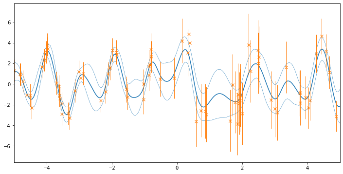
Questions for the reader

1. What is the difference in meaning between the orange vertical bars and the blue regions in the prediction?

2. Why did we not implement _conditional_mean and _conditional_variance in the HeteroskedasticGaussian likelihood? What could be done here?

3. What are some better kernel settings for this dataset? How could they be estimated?

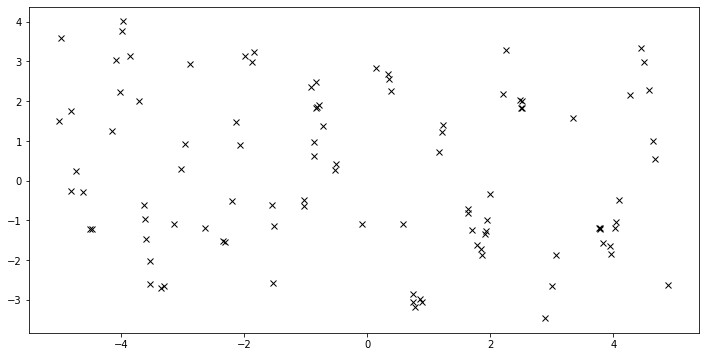
Demo 2: grouped noise variances

In this demo, we won’t assume that the noise variances are known, but we will assume that they’re known in two groups. This example represents a case where we might know that an instrument has varying fidelity for different regions, but we do not know what those fidelities are.

Of course it would be straightforward to add more groups, or even one group per data point. We’ll stick with two for simplicity.

np.random.seed(1)  # for reproducibility and to make it independent from demo 1

Generate data

def generate_data(N=100):
    X = np.random.rand(N)[:, None] * 10 - 5  # Inputs, shape N x 1
    F = 2.5 * np.sin(6 * X) + np.cos(3 * X)  # Mean function values
    groups = np.where(X > 0, 0, 1)
    NoiseVar = np.array([0.02, 0.5])[groups]  # Different variances for the two groups
    Y = F + np.random.randn(N, 1) * np.sqrt(NoiseVar)  # Noisy data
    return X, Y, groups


X, Y, groups = generate_data()

# here's a plot of the raw data.
fig, ax = plt.subplots(1, 1, figsize=(12, 6))
_ = ax.plot(X, Y, "kx")

Data structure

In this case, we need to let the model know which group each data point belongs to. We’ll use a similar trick to the above, stacking the group identifier with the data:

Y_data = np.hstack([Y, groups])

Build a likelihood

This time, we’ll use a builtin likelihood, SwitchedLikelihood, which is a container for other likelihoods, and applies them to the first Y_data column depending on the index in the second. We’re able to access and optimize the parameters of those likelihoods. Here, we’ll (incorrectly) initialize the variances of our likelihoods to 1, to demonstrate how we can recover reasonable values for these through maximum-likelihood estimation.

likelihood = gpflow.likelihoods.SwitchedLikelihood(
    [gpflow.likelihoods.Gaussian(variance=1.0), gpflow.likelihoods.Gaussian(variance=1.0)]
)

# model construction (notice that num_latent_gps is 1)
kernel = gpflow.kernels.Matern52(lengthscales=0.5)
model = gpflow.models.VGP((X, Y_data), kernel=kernel, likelihood=likelihood, num_latent_gps=1)

for _ in range(ci_niter(1000)):
    natgrad.minimize(model.training_loss, [(model.q_mu, model.q_sqrt)])

We’ve now fitted the VGP model to the data, but without optimizing over the hyperparameters. Plotting the data, we see that the fit is not terrible, but hasn’t made use of our knowledge of the varying noise.

# let's do some plotting!
xx = np.linspace(-5, 5, 200)[:, None]

mu, var = model.predict_f(xx)

fig, ax = plt.subplots(1, 1, figsize=(12, 6))
ax.plot(xx, mu, "C0")
ax.plot(xx, mu + 2 * np.sqrt(var), "C0", lw=0.5)
ax.plot(xx, mu - 2 * np.sqrt(var), "C0", lw=0.5)

ax.plot(X, Y, "C1x", mew=2)
_ = ax.set_xlim(-5, 5)

Optimizing the noise variances

Here we’ll optimize over both the noise variance and the variational parameters, applying natural gradients interleaved with the Adam optimizer.

As before, we mark the variational parameters as not trainable, in order to train them separately with the natural gradient method.

likelihood = gpflow.likelihoods.SwitchedLikelihood(
    [gpflow.likelihoods.Gaussian(variance=1.0), gpflow.likelihoods.Gaussian(variance=1.0)]
)
kernel = gpflow.kernels.Matern52(lengthscales=0.5)
model = gpflow.models.VGP((X, Y_data), kernel=kernel, likelihood=likelihood, num_latent_gps=1)

set_trainable(model.q_mu, False)
set_trainable(model.q_sqrt, False)

for _ in range(ci_niter(1000)):
    natgrad.minimize(model.training_loss, [(model.q_mu, model.q_sqrt)])
    adam.minimize(model.training_loss, model.trainable_variables)

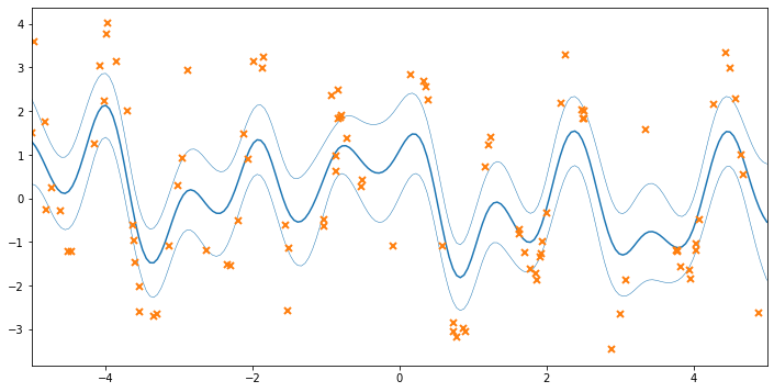
Plotting the fitted model

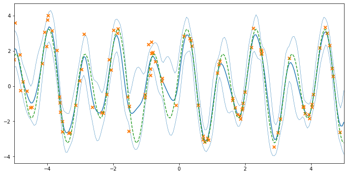
Now that the noise variances have been estimated, we can see the final model fit. The predictive variance is higher on the left side of the plot, where we know that the data have different variance. We’ll plot the known underlying function in green to see how effectively we’ve recovered the ground truth. We can also print the model to examine the estimated noise variances:

# let's do some plotting!
xx = np.linspace(-5, 5, 200)[:, None]

mu, var = model.predict_f(xx)

fig, ax = plt.subplots(1, 1, figsize=(12, 6))
ax.plot(xx, mu, "C0")
ax.plot(xx, mu + 2 * np.sqrt(var), "C0", lw=0.5)
ax.plot(xx, mu - 2 * np.sqrt(var), "C0", lw=0.5)

ax.plot(X, Y, "C1x", mew=2)
ax.set_xlim(-5, 5)
_ = ax.plot(xx, 2.5 * np.sin(6 * xx) + np.cos(3 * xx), "C2--")

from gpflow.utilities import print_summary

print_summary(model, fmt="notebook")

name	class	transform	prior	trainable	shape	dtype	value
VGP.kernel.variance	Parameter	Softplus		True	()	float64	2.048774633510034
VGP.kernel.lengthscales	Parameter	Softplus		True	()	float64	0.2174351066754893
VGP.likelihood.likelihoods[0].variance	Parameter	Softplus + Shift		True	()	float64	0.29148168577591166
VGP.likelihood.likelihoods[1].variance	Parameter	Softplus + Shift		True	()	float64	0.6055446990450548
VGP.num_data	Parameter	Identity		False	()	int32	100
VGP.q_mu	Parameter	Identity		False	(100, 1)	float64	[[1.15102310e+00...
VGP.q_sqrt	Parameter	FillTriangular		False	(1, 100, 100)	float64	[[[2.06898404e-01, 0.00000000e+00, 0.00000000e+00...

Further reading

To model the variance using a second GP, see the Heteroskedastic regression notebook.