Monitoring Optimisation

In this notebook we cover how to monitor the model and certain metrics during optimisation.

Setup

import numpy as np
import matplotlib.pyplot as plt
import tensorflow as tf

import gpflow
from gpflow.ci_utils import ci_niter

np.random.seed(0)

The monitoring functionality lives in gpflow.monitor. For now, we import ModelToTensorBoard, ImageToTensorBoard, ScalarToTensorBoard monitoring tasks and MonitorTaskGroup and Monitor.

from gpflow.monitor import (
    ImageToTensorBoard,
    ModelToTensorBoard,
    Monitor,
    MonitorTaskGroup,
    ScalarToTensorBoard,
)

Set up data and model

# Define some configuration constants.

num_data = 100
noise_std = 0.1
optimisation_steps = ci_niter(100)

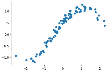
# Create dummy data.

X = np.random.randn(num_data, 1)  # [N, 2]
Y = np.sin(X) + 0.5 * np.cos(X) + np.random.randn(*X.shape) * noise_std  # [N, 1]
plt.plot(X, Y, "o")

[<matplotlib.lines.Line2D at 0x7fbc74cf3e80>]

# Set up model and print

kernel = gpflow.kernels.SquaredExponential(lengthscales=[1.0, 2.0]) + gpflow.kernels.Linear()
model = gpflow.models.GPR((X, Y), kernel, noise_variance=noise_std ** 2)
model

2022-03-18 10:10:19.843896: I tensorflow/stream_executor/cuda/cuda_gpu_executor.cc:936] successful NUMA node read from SysFS had negative value (-1), but there must be at least one NUMA node, so returning NUMA node zero
2022-03-18 10:10:19.847104: W tensorflow/stream_executor/platform/default/dso_loader.cc:64] Could not load dynamic library 'libcusolver.so.11'; dlerror: libcusolver.so.11: cannot open shared object file: No such file or directory
2022-03-18 10:10:19.847662: W tensorflow/core/common_runtime/gpu/gpu_device.cc:1850] Cannot dlopen some GPU libraries. Please make sure the missing libraries mentioned above are installed properly if you would like to use GPU. Follow the guide at https://www.tensorflow.org/install/gpu for how to download and setup the required libraries for your platform.
Skipping registering GPU devices...
2022-03-18 10:10:19.848452: I tensorflow/core/platform/cpu_feature_guard.cc:151] This TensorFlow binary is optimized with oneAPI Deep Neural Network Library (oneDNN) to use the following CPU instructions in performance-critical operations:  AVX2 FMA
To enable them in other operations, rebuild TensorFlow with the appropriate compiler flags.

<gpflow.models.gpr.GPR object at 0x7fbc74d337c0>

name	class	transform	prior	trainable	shape	dtype	value
GPR.kernel.kernels[0].variance	Parameter	Softplus		True	()	float64	1.0
GPR.kernel.kernels[0].lengthscales	Parameter	Softplus		True	(2,)	float64	[1. 2.]
GPR.kernel.kernels[1].variance	Parameter	Softplus		True	()	float64	1.0
GPR.likelihood.variance	Parameter	Softplus + Shift		True	()	float64	0.009999999999999998

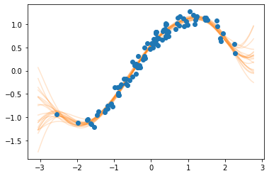
# We define a function that plots the model's prediction (in the form of samples) together with the data.
# Importantly, this function has no other argument than `fig: matplotlib.figure.Figure` and `ax: matplotlib.figure.Axes`.


def plot_prediction(fig, ax):
    Xnew = np.linspace(X.min() - 0.5, X.max() + 0.5, 100).reshape(-1, 1)
    Ypred = model.predict_f_samples(Xnew, full_cov=True, num_samples=20)
    ax.plot(Xnew.flatten(), np.squeeze(Ypred).T, "C1", alpha=0.2)
    ax.plot(X, Y, "o")


# Let's check if the function does the desired plotting
fig = plt.figure()
ax = fig.subplots()
plot_prediction(fig, ax)
plt.show()

Set up monitoring tasks

We now define the MonitorTasks that will be executed during the optimisation. For this tutorial we set up three tasks: - ModelToTensorBoard: writes the models hyper-parameters such as likelihood.variance and kernel.lengthscales to a TensorBoard. - ImageToTensorBoard: writes custom matplotlib images to a TensorBoard. - ScalarToTensorBoard: writes any scalar value to a TensorBoard. Here, we use it to write the model’s training objective.

log_dir = "logs"  # Directory where TensorBoard files will be written.
model_task = ModelToTensorBoard(log_dir, model)
image_task = ImageToTensorBoard(log_dir, plot_prediction, "image_samples")
lml_task = ScalarToTensorBoard(log_dir, lambda: model.training_loss(), "training_objective")

We now group the tasks in a set of fast and slow tasks and pass them to the monitor. This allows us to execute the groups at a different frequency.

# Plotting tasks can be quite slow. We want to run them less frequently.
# We group them in a `MonitorTaskGroup` and set the period to 5.
slow_tasks = MonitorTaskGroup(image_task, period=5)

# The other tasks are fast. We run them at each iteration of the optimisation.
fast_tasks = MonitorTaskGroup([model_task, lml_task], period=1)

# Both groups are passed to the monitor.
# `slow_tasks` will be run five times less frequently than `fast_tasks`.
monitor = Monitor(fast_tasks, slow_tasks)

training_loss = model.training_loss_closure(
    compile=True
)  # compile=True (default): compiles using tf.function
opt = tf.optimizers.Adam()

for step in range(optimisation_steps):
    opt.minimize(training_loss, model.trainable_variables)
    monitor(step)  # <-- run the monitoring

2022-03-18 10:10:20.105715: W tensorflow/python/util/util.cc:368] Sets are not currently considered sequences, but this may change in the future, so consider avoiding using them.

TensorBoard is accessible through the browser, after launching the server by running tensorboard --logdir ${logdir}. See the TensorFlow documentation on TensorBoard for more information.

For optimal performance, we can also wrap the monitor call inside tf.function:

opt = tf.optimizers.Adam()

log_dir_compiled = f"{log_dir}/compiled"
model_task = ModelToTensorBoard(log_dir_compiled, model)
lml_task = ScalarToTensorBoard(
    log_dir_compiled, lambda: model.training_loss(), "training_objective"
)
# Note that the `ImageToTensorBoard` task cannot be compiled, and is omitted from the monitoring
monitor = Monitor(MonitorTaskGroup([model_task, lml_task]))

In the optimisation loop below we use tf.range (rather than Python’s built-in range) to avoid re-tracing the step function each time.

@tf.function
def step(i):
    opt.minimize(model.training_loss, model.trainable_variables)
    monitor(i)


# Notice the tf.range
for i in tf.range(optimisation_steps):
    step(i)

When opening TensorBoard, you may need to use the command tensorboard --logdir . --reload_multifile=true, as multiple FileWriter objects are used.

Scipy Optimization monitoring

Note that if you want to use the Scipy optimizer provided by GPflow, and want to monitor the training progress, then you need to simply replace the optimization loop with a single call to its minimize method and pass in the monitor as a step_callback keyword argument:

opt = gpflow.optimizers.Scipy()

log_dir_scipy = f"{log_dir}/scipy"
model_task = ModelToTensorBoard(log_dir_scipy, model)
lml_task = ScalarToTensorBoard(log_dir_scipy, lambda: model.training_loss(), "training_objective")
image_task = ImageToTensorBoard(log_dir_scipy, plot_prediction, "image_samples")

monitor = Monitor(
    MonitorTaskGroup([model_task, lml_task], period=1), MonitorTaskGroup(image_task, period=5)
)

opt.minimize(training_loss, model.trainable_variables, step_callback=monitor)

      fun: -69.68099880887888
 hess_inv: <5x5 LbfgsInvHessProduct with dtype=float64>
      jac: array([-2.96735852e-04, -4.30340682e-04,  3.97824556e-04,  2.26011878e-06,
        4.29130061e-04])
  message: 'CONVERGENCE: REL_REDUCTION_OF_F_<=_FACTR*EPSMCH'
     nfev: 37
      nit: 28
     njev: 37
   status: 0
  success: True
        x: array([  2.07005974,   1.74612939,   0.18194305, -15.21874538,
        -4.53840856])