Bayesian Gaussian process latent variable model (Bayesian GPLVM)

This notebook shows how to use the Bayesian GPLVM model. This is an unsupervised learning method usually used for dimensionality reduction. For an in-depth overview of GPLVMs,see [1, 2].

import gpflow
import numpy as np

import matplotlib.pyplot as plt
import tensorflow as tf

import gpflow
from gpflow.utilities import ops, print_summary
from gpflow.config import set_default_float, default_float, set_default_summary_fmt
from gpflow.ci_utils import ci_niter

set_default_float(np.float64)
set_default_summary_fmt("notebook")

%matplotlib inline

Data

We are using the “three phase oil flow” dataset used initially for demonstrating the Generative Topographic mapping from [3].

data = np.load("./data/three_phase_oil_flow.npz")

Following the GPflow notation we assume this dataset has a shape of [num_data, output_dim]

Y = tf.convert_to_tensor(data["Y"], dtype=default_float())

2022-03-18 10:10:06.139485: I tensorflow/stream_executor/cuda/cuda_gpu_executor.cc:936] successful NUMA node read from SysFS had negative value (-1), but there must be at least one NUMA node, so returning NUMA node zero
2022-03-18 10:10:06.142845: W tensorflow/stream_executor/platform/default/dso_loader.cc:64] Could not load dynamic library 'libcusolver.so.11'; dlerror: libcusolver.so.11: cannot open shared object file: No such file or directory
2022-03-18 10:10:06.143389: W tensorflow/core/common_runtime/gpu/gpu_device.cc:1850] Cannot dlopen some GPU libraries. Please make sure the missing libraries mentioned above are installed properly if you would like to use GPU. Follow the guide at https://www.tensorflow.org/install/gpu for how to download and setup the required libraries for your platform.
Skipping registering GPU devices...
2022-03-18 10:10:06.143868: I tensorflow/core/platform/cpu_feature_guard.cc:151] This TensorFlow binary is optimized with oneAPI Deep Neural Network Library (oneDNN) to use the following CPU instructions in performance-critical operations:  AVX2 FMA
To enable them in other operations, rebuild TensorFlow with the appropriate compiler flags.

Integer in \([0, 2]\) indicating to which class the data point belongs (shape [num_data,]). Not used for model fitting, only for plotting afterwards.

labels = tf.convert_to_tensor(data["labels"])

print("Number of points: {} and Number of dimensions: {}".format(Y.shape[0], Y.shape[1]))

Number of points: 100 and Number of dimensions: 12

Model construction

We start by initializing the required variables:

latent_dim = 2  # number of latent dimensions
num_inducing = 20  # number of inducing pts
num_data = Y.shape[0]  # number of data points

Initialize via PCA:

X_mean_init = ops.pca_reduce(Y, latent_dim)
X_var_init = tf.ones((num_data, latent_dim), dtype=default_float())

Pick inducing inputs randomly from dataset initialization:

np.random.seed(1)  # for reproducibility
inducing_variable = tf.convert_to_tensor(
    np.random.permutation(X_mean_init.numpy())[:num_inducing], dtype=default_float()
)

We construct a Squared Exponential (SE) kernel operating on the two-dimensional latent space. The ARD parameter stands for Automatic Relevance Determination, which in practice means that we learn a different lengthscale for each of the input dimensions. See Manipulating kernels for more information.

lengthscales = tf.convert_to_tensor([1.0] * latent_dim, dtype=default_float())
kernel = gpflow.kernels.RBF(lengthscales=lengthscales)

We have all the necessary ingredients to construct the model. GPflow contains an implementation of the Bayesian GPLVM:

gplvm = gpflow.models.BayesianGPLVM(
    Y,
    X_data_mean=X_mean_init,
    X_data_var=X_var_init,
    kernel=kernel,
    inducing_variable=inducing_variable,
)
# Instead of passing an inducing_variable directly, we can also set the num_inducing_variables argument to an integer, which will randomly pick from the data.

We change the default likelihood variance, which is 1, to 0.01.

gplvm.likelihood.variance.assign(0.01)

<tf.Variable 'UnreadVariable' shape=() dtype=float64, numpy=-4.600266525158521>

Next we optimize the created model. Given that this model has a deterministic evidence lower bound (ELBO), we can use SciPy’s BFGS optimizer.

opt = gpflow.optimizers.Scipy()
maxiter = ci_niter(1000)
_ = opt.minimize(
    gplvm.training_loss,
    method="BFGS",
    variables=gplvm.trainable_variables,
    options=dict(maxiter=maxiter),
)

2022-03-18 10:10:06.248643: W tensorflow/python/util/util.cc:368] Sets are not currently considered sequences, but this may change in the future, so consider avoiding using them.

Model analysis

GPflow allows you to inspect the learned model hyperparameters.

print_summary(gplvm)

name	class	transform	prior	trainable	shape	dtype	value
BayesianGPLVM.kernel.variance	Parameter	Softplus		True	()	float64	0.918006903235084
BayesianGPLVM.kernel.lengthscales	Parameter	Softplus		True	(2,)	float64	[0.86660903 1.76001201]
BayesianGPLVM.likelihood.variance	Parameter	Softplus + Shift		True	()	float64	0.006477224413046602
BayesianGPLVM.X_data_mean	Parameter	Identity		True	(100, 2)	float64	[[-7.98739699e-01, 3.04430690e+00...
BayesianGPLVM.X_data_var	Parameter	Softplus		True	(100, 2)	float64	[[0.00040638, 0.00153666...
BayesianGPLVM.inducing_variable.Z	Parameter	Identity		True	(20, 2)	float64	[[1.31766414e+00, -1.72368420e+00...

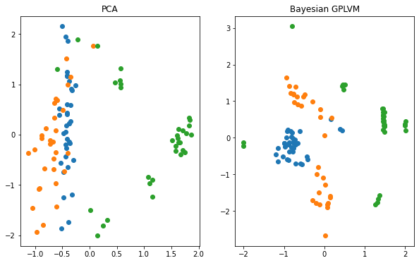
Plotting vs. Principle Component Analysis (PCA)

The reduction of the dimensionality of the dataset to two dimensions allows us to visualize the learned manifold. We compare the Bayesian GPLVM’s latent space to the deterministic PCA’s one.

X_pca = ops.pca_reduce(Y, latent_dim).numpy()
gplvm_X_mean = gplvm.X_data_mean.numpy()

f, ax = plt.subplots(1, 2, figsize=(10, 6))

for i in np.unique(labels):
    ax[0].scatter(X_pca[labels == i, 0], X_pca[labels == i, 1], label=i)
    ax[1].scatter(gplvm_X_mean[labels == i, 0], gplvm_X_mean[labels == i, 1], label=i)
    ax[0].set_title("PCA")
    ax[1].set_title("Bayesian GPLVM")

References

[1] Lawrence, Neil D. ‘Gaussian process latent variable models for visualization of high dimensional data’. Advances in Neural Information Processing Systems. 2004.

[2] Titsias, Michalis, and Neil D. Lawrence. ‘Bayesian Gaussian process latent variable model’. Proceedings of the Thirteenth International Conference on Artificial Intelligence and Statistics. 2010.

[3] Bishop, Christopher M., and Gwilym D. James. ‘Analysis of multiphase flows using dual-energy gamma densitometry and neural networks’. Nuclear Instruments and Methods in Physics Research Section A: Accelerators, Spectrometers, Detectors and Associated Equipment 327.2-3 (1993): 580-593.