Multi-output Gaussian processes in GPflow#

This notebook shows how to construct a multi-output GP model using GPflow, together with different interdomain inducing variables which lead to different approximation properties. GPflow provides a framework for specifying multioutput GP priors, and interdomain approximations which is - modular, by providing a consistent interface for the user of the resulting SVGP model, - extensible, by allowing new interdomain variables and kernels to be specified while reusing exising code where possible, - efficient, by allowing the most efficient custom code path to be specified where desired.

Getting to grips with the maths and code can be a bit daunting, so to accompany the documentation there is an in-depth review on arXiv, which provides a unified mathematical framework, together with a high-level description of software design choices in GPflow.

This notebook shows the various design choices that can be made, to show the reader the flexibility of the framework. This is done in the hope that an example is provided that can be easily adapted to the special case that the reader wants to implement.

A reader who just wants to use a multioutput kernel should simply choose the most efficient set of inducing variables.

To cite this framework, please reference our arXiv paper.

@article{GPflow2020multioutput,
  author = {{van der Wilk}, Mark and Dutordoir, Vincent and John, ST and
            Artemev, Artem and Adam, Vincent and Hensman, James},
  title = {A Framework for Interdomain and Multioutput {G}aussian Processes},
  year = {2020},
  journal = {arXiv:2003.01115},
  url = {https://arxiv.org/abs/2003.01115}
}

\begin{equation} \newcommand{\GP}{\mathcal{GP}} \newcommand{\NN}{\mathcal{N}} \newcommand{\LL}{\mathcal{L}} \newcommand{\RR}{\mathbb{R}} \newcommand{\EE}{\mathbb{E}} \newcommand{\valpha}{\boldsymbol\alpha} \newcommand{\vf}{\mathbf{f}} \newcommand{\vF}{\mathbf{F}} \newcommand{\vg}{\mathbf{g}} \newcommand{\vW}{\mathbf{W}} \newcommand{\vI}{\mathbf{I}} \newcommand{\vZ}{\mathbf{Z}} \newcommand{\vu}{\mathbf{u}} \newcommand{\vU}{\mathbf{U}} \newcommand{\vX}{\mathbf{X}} \newcommand{\vY}{\mathbf{Y}} \newcommand{\identity}{\mathbb{I}} \end{equation}

Task#

We will consider a regression problem for functions \(f: \mathbb{R}^D \rightarrow \mathbb{R}^P\). We assume that the dataset is of the form \((X, f_1), \dots, (X, f_P)\), that is, we observe all the outputs for a particular input location (for cases where there are not fully observed outputs for each input, see A simple demonstration of coregionalization).

Here we assume a model of the form: \begin{equation} f(x) = W g(x), \end{equation} where \(g(x) \in \mathbb{R}^L\), \(f(x) \in \mathbb{R}^P\) and \(W \in \mathbb{R}^{P \times L}\). We assume that the outputs of \(g\) are uncorrelated, and that by mixing them with \(W\) they become correlated. In this notebook, we show how to build this model using Sparse Variational Gaussian Process (SVGP) for \(g\), which scales well with the numbers of data points and outputs.

Here we have two options for \(g\): 1. The output dimensions of \(g\) share the same kernel. 2. Each output of \(g\) has a separate kernel.

In addition, we have two further suboptions for the inducing inputs of \(g\): 1. The instances of \(g\) share the same inducing inputs. 2. Each output of \(g\) has its own set of inducing inputs.

The notation is as follows: - \(X \in \mathbb{R}^{N \times D}\) denotes the input - \(Y \in \RR^{N \times P}\) denotes the output - \(k_{1..L}\), \(L\) are kernels on \(\RR^{N \times D}\) - \(g_{1..L}\), \(L\) are independent \(\GP\)s with \(g_l \sim \GP(0,k_l)\) - \(f_{1..P}\), \(P\) are correlated \(\GP\)s with \(\vf = \vW \vg\)

[1]:

import matplotlib.pyplot as plt
import numpy as np

import gpflow as gpf
from gpflow.ci_utils import reduce_in_tests
from gpflow.utilities import print_summary

gpf.config.set_default_float(np.float64)
gpf.config.set_default_summary_fmt("notebook")
np.random.seed(0)
%matplotlib inline

MAXITER = reduce_in_tests(2000)

2024-02-07 11:46:05.249156: I external/local_tsl/tsl/cuda/cudart_stub.cc:31] Could not find cuda drivers on your machine, GPU will not be used.
2024-02-07 11:46:05.292392: E external/local_xla/xla/stream_executor/cuda/cuda_dnn.cc:9261] Unable to register cuDNN factory: Attempting to register factory for plugin cuDNN when one has already been registered
2024-02-07 11:46:05.292427: E external/local_xla/xla/stream_executor/cuda/cuda_fft.cc:607] Unable to register cuFFT factory: Attempting to register factory for plugin cuFFT when one has already been registered
2024-02-07 11:46:05.293833: E external/local_xla/xla/stream_executor/cuda/cuda_blas.cc:1515] Unable to register cuBLAS factory: Attempting to register factory for plugin cuBLAS when one has already been registered
2024-02-07 11:46:05.301257: I external/local_tsl/tsl/cuda/cudart_stub.cc:31] Could not find cuda drivers on your machine, GPU will not be used.
2024-02-07 11:46:05.301750: I tensorflow/core/platform/cpu_feature_guard.cc:182] This TensorFlow binary is optimized to use available CPU instructions in performance-critical operations.
To enable the following instructions: AVX2 AVX512F FMA, in other operations, rebuild TensorFlow with the appropriate compiler flags.

2024-02-07 11:46:06.508431: W tensorflow/compiler/tf2tensorrt/utils/py_utils.cc:38] TF-TRT Warning: Could not find TensorRT

Generate synthetic data#

We create a utility function to generate synthetic data. We assume that:

[2]:

N = 100  # number of points
D = 1  # number of input dimensions
M = 15  # number of inducing points
L = 2  # number of latent GPs
P = 3  # number of observations = output dimensions

[3]:

def generate_data(N=100):
    X = np.random.rand(N)[:, None] * 10 - 5  # Inputs = N x D
    G = np.hstack((0.5 * np.sin(3 * X) + X, 3.0 * np.cos(X) - X))  # G = N x L
    W = np.array([[0.5, -0.3, 1.5], [-0.4, 0.43, 0.0]])  # L x P
    F = np.matmul(G, W)  # N x P
    Y = F + np.random.randn(*F.shape) * [0.2, 0.2, 0.2]

    return X, Y

[4]:

X, Y = data = generate_data(N)
Zinit = np.linspace(-5, 5, M)[:, None]

We create a utility function for plotting:

[5]:

def plot_model(m, lower=-8.0, upper=8.0):
    pX = np.linspace(lower, upper, 100)[:, None]
    pY, pYv = m.predict_y(pX)
    if pY.ndim == 3:
        pY = pY[:, 0, :]
    plt.plot(X, Y, "x")
    plt.gca().set_prop_cycle(None)
    plt.plot(pX, pY)
    for i in range(pY.shape[1]):
        top = pY[:, i] + 2.0 * pYv[:, i] ** 0.5
        bot = pY[:, i] - 2.0 * pYv[:, i] ** 0.5
        plt.fill_between(pX[:, 0], top, bot, alpha=0.3)
    plt.xlabel("X")
    plt.ylabel("f")
    plt.title(f"ELBO: {m.elbo(data):.3}")
    plt.plot(Z, Z * 0.0, "o")

Model the outputs of \(f(x)\) directly#

The three following examples show how to model the outputs of the model \(f(x)\) directly. Mathematically, this case is equivalent to having: \begin{equation} f(x) = I g(x), \end{equation} i.e. \(W = I\) and \(P = L\).

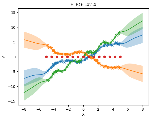
1. Shared independent multi-output kernel (MOK) and shared independent inducing variables#

Here the priors on all outputs are constrained to have the same kernel hyperparameters. We also share the inducing inputs between all outputs. The different GPs are independent both in the prior and the approximate posterior.

[6]:

# create multi-output kernel
kernel = gpf.kernels.SharedIndependent(
    gpf.kernels.SquaredExponential() + gpf.kernels.Linear(), output_dim=P
)
# initialization of inducing input locations (M random points from the training inputs)
Z = Zinit.copy()
# create multi-output inducing variables from Z
iv = gpf.inducing_variables.SharedIndependentInducingVariables(
    gpf.inducing_variables.InducingPoints(Z)
)

[7]:

# create SVGP model as usual and optimize
m = gpf.models.SVGP(
    kernel, gpf.likelihoods.Gaussian(), inducing_variable=iv, num_latent_gps=P
)
print_summary(m)

name	class	transform	trainable	shape	dtype	value
SVGP.kernel.kernel.kernels[0].variance	Parameter	Softplus	True	()	float64	1.0
SVGP.kernel.kernel.kernels[0].lengthscales	Parameter	Softplus	True	()	float64	1.0
SVGP.kernel.kernel.kernels[1].variance	Parameter	Softplus	True	()	float64	1.0
SVGP.likelihood.variance	Parameter	Softplus + Shift	True	()	float64	1.0
SVGP.inducing_variable.inducing_variable.Z	Parameter	Identity	True	(15, 1)	float64	[[-5....
SVGP.q_mu	Parameter	Identity	True	(15, 3)	float64	[[0., 0., 0....
SVGP.q_sqrt	Parameter	FillTriangular	True	(3, 15, 15)	float64	[[[1., 0., 0....

[8]:

def optimize_model_with_scipy(model):
    optimizer = gpf.optimizers.Scipy()
    optimizer.minimize(
        model.training_loss_closure(data),
        variables=model.trainable_variables,
        method="l-bfgs-b",
        options={"disp": 50, "maxiter": MAXITER},
    )


optimize_model_with_scipy(m)

 This problem is unconstrained.

RUNNING THE L-BFGS-B CODE

           * * *

Machine precision = 2.220D-16
 N =          424     M =           10

At X0         0 variables are exactly at the bounds

At iterate    0    f=  3.26251D+03    |proj g|=  1.79322D+03

At iterate   50    f=  1.60046D+02    |proj g|=  2.23880D+01

At iterate  100    f=  6.25440D+01    |proj g|=  2.71497D+01


At iterate  150    f=  5.45593D+01    |proj g|=  2.85566D+01

At iterate  200    f=  5.04417D+01    |proj g|=  2.36414D+01

At iterate  250    f=  4.81566D+01    |proj g|=  7.56354D+00


At iterate  300    f=  4.66562D+01    |proj g|=  1.54605D+01

At iterate  350    f=  4.55273D+01    |proj g|=  9.03129D+00

At iterate  400    f=  4.46163D+01    |proj g|=  1.82533D+00

At iterate  450    f=  4.37082D+01    |proj g|=  3.70951D+00


At iterate  500    f=  4.30992D+01    |proj g|=  4.54184D+00

At iterate  550    f=  4.27762D+01    |proj g|=  6.18559D+00

At iterate  600    f=  4.26316D+01    |proj g|=  1.16861D+00

At iterate  650    f=  4.25440D+01    |proj g|=  3.02942D+00


At iterate  700    f=  4.24932D+01    |proj g|=  2.39140D+00

At iterate  750    f=  4.24607D+01    |proj g|=  1.04215D+00

At iterate  800    f=  4.24441D+01    |proj g|=  5.39999D-01

At iterate  850    f=  4.24361D+01    |proj g|=  5.50694D-01


At iterate  900    f=  4.24318D+01    |proj g|=  2.55596D-01

At iterate  950    f=  4.24281D+01    |proj g|=  5.87821D-01

At iterate 1000    f=  4.24261D+01    |proj g|=  2.00414D-01

At iterate 1050    f=  4.24247D+01    |proj g|=  1.17232D-01


At iterate 1100    f=  4.24240D+01    |proj g|=  7.82463D-02

At iterate 1150    f=  4.24236D+01    |proj g|=  2.26153D-01

At iterate 1200    f=  4.24231D+01    |proj g|=  5.70376D-01

At iterate 1250    f=  4.24227D+01    |proj g|=  1.57686D-01


At iterate 1300    f=  4.24223D+01    |proj g|=  1.62637D-01

At iterate 1350    f=  4.24219D+01    |proj g|=  9.75631D-02

At iterate 1400    f=  4.24215D+01    |proj g|=  1.13964D-01

At iterate 1450    f=  4.24211D+01    |proj g|=  1.16687D-01


At iterate 1500    f=  4.24209D+01    |proj g|=  5.41853D-02

At iterate 1550    f=  4.24208D+01    |proj g|=  6.38099D-02

At iterate 1600    f=  4.24206D+01    |proj g|=  1.29858D-01

At iterate 1650    f=  4.24205D+01    |proj g|=  8.11513D-02


At iterate 1700    f=  4.24205D+01    |proj g|=  4.87641D-02

           * * *

Tit   = total number of iterations
Tnf   = total number of function evaluations
Tnint = total number of segments explored during Cauchy searches
Skip  = number of BFGS updates skipped
Nact  = number of active bounds at final generalized Cauchy point
Projg = norm of the final projected gradient
F     = final function value

           * * *

   N    Tit     Tnf  Tnint  Skip  Nact     Projg        F
  424   1709   1835      1     0     0   1.169D-02   4.242D+01
  F =   42.420488076940394

CONVERGENCE: REL_REDUCTION_OF_F_<=_FACTR*EPSMCH

[9]:

print_summary(m)

name	class	transform	trainable	shape	dtype	value
SVGP.kernel.kernel.kernels[0].variance	Parameter	Softplus	True	()	float64	0.9280167114500715
SVGP.kernel.kernel.kernels[0].lengthscales	Parameter	Softplus	True	()	float64	0.7984037597218473
SVGP.kernel.kernel.kernels[1].variance	Parameter	Softplus	True	()	float64	1.21214
SVGP.likelihood.variance	Parameter	Softplus + Shift	True	()	float64	0.039659901213752305
SVGP.inducing_variable.inducing_variable.Z	Parameter	Identity	True	(15, 1)	float64	[[-4.83956...
SVGP.q_mu	Parameter	Identity	True	(15, 3)	float64	[[-0.90158021, 0.69899149, -1.47493...
SVGP.q_sqrt	Parameter	FillTriangular	True	(3, 15, 15)	float64	[[[1.71237154e-02, 0.00000000e+00, 0.00000000e+00...

[10]:

# Plot predictions and observations
plot_model(m)

../../_images/notebooks_advanced_multioutput_15_0.png

[11]:

print_summary(m.kernel)
m.kernel.kernel.kernels[0].lengthscales

name	class	transform	trainable	shape	dtype	value
SharedIndependent.kernel.kernels[0].variance	Parameter	Softplus	True	()	float64	0.928017
SharedIndependent.kernel.kernels[0].lengthscales	Parameter	Softplus	True	()	float64	0.798404
SharedIndependent.kernel.kernels[1].variance	Parameter	Softplus	True	()	float64	1.21214

[11]:

<Parameter: name=softplus, dtype=float64, shape=[], fn="softplus", numpy=0.7984037597218473>

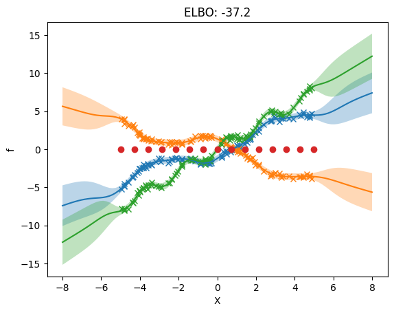
2. Separate independent MOK and shared independent inducing variables#

Here we allow different hyperparameters for the priors of each output. We still share the inducing inputs between all outputs.

[12]:

# Create list of kernels for each output
kern_list = [
    gpf.kernels.SquaredExponential() + gpf.kernels.Linear() for _ in range(P)
]
# Create multi-output kernel from kernel list
kernel = gpf.kernels.SeparateIndependent(kern_list)
# initialization of inducing input locations (M random points from the training inputs)
Z = Zinit.copy()
# create multi-output inducing variables from Z
iv = gpf.inducing_variables.SharedIndependentInducingVariables(
    gpf.inducing_variables.InducingPoints(Z)
)

[13]:

# create SVGP model as usual and optimize
m = gpf.models.SVGP(
    kernel, gpf.likelihoods.Gaussian(), inducing_variable=iv, num_latent_gps=P
)

[14]:

optimize_model_with_scipy(m)

WARNING:tensorflow:From /tmp/max_venv/lib/python3.11/site-packages/tensorflow/python/util/deprecation.py:660: calling map_fn_v2 (from tensorflow.python.ops.map_fn) with dtype is deprecated and will be removed in a future version.
Instructions for updating:
Use fn_output_signature instead

 This problem is unconstrained.

RUNNING THE L-BFGS-B CODE

           * * *

Machine precision = 2.220D-16
 N =          430     M =           10

At X0         0 variables are exactly at the bounds

At iterate    0    f=  3.26251D+03    |proj g|=  1.79322D+03


At iterate   50    f=  1.94337D+02    |proj g|=  7.19162D+00


At iterate  100    f=  1.61420D+02    |proj g|=  9.22259D+01


At iterate  150    f=  5.98686D+01    |proj g|=  4.94480D+01

At iterate  200    f=  4.98426D+01    |proj g|=  4.40224D+01


At iterate  250    f=  4.66400D+01    |proj g|=  6.64269D+00


At iterate  300    f=  4.47472D+01    |proj g|=  3.01200D+01

At iterate  350    f=  4.35825D+01    |proj g|=  2.66816D+01


At iterate  400    f=  4.18951D+01    |proj g|=  1.87723D+01


At iterate  450    f=  4.02256D+01    |proj g|=  1.97700D+01

At iterate  500    f=  3.92505D+01    |proj g|=  8.13694D+00


At iterate  550    f=  3.86248D+01    |proj g|=  2.45805D+00

At iterate  600    f=  3.82643D+01    |proj g|=  9.98024D+00


At iterate  650    f=  3.79192D+01    |proj g|=  3.54551D+00

At iterate  700    f=  3.76512D+01    |proj g|=  2.72885D+00


At iterate  750    f=  3.74929D+01    |proj g|=  2.07019D+00

At iterate  800    f=  3.74003D+01    |proj g|=  1.27696D+00


At iterate  850    f=  3.73412D+01    |proj g|=  1.00416D+00

At iterate  900    f=  3.73078D+01    |proj g|=  9.49059D-01


At iterate  950    f=  3.72798D+01    |proj g|=  3.28321D+00


At iterate 1000    f=  3.72634D+01    |proj g|=  6.53366D-01


At iterate 1050    f=  3.72504D+01    |proj g|=  1.47493D+00


At iterate 1100    f=  3.72385D+01    |proj g|=  6.01080D-01

At iterate 1150    f=  3.72289D+01    |proj g|=  2.23900D+00


At iterate 1200    f=  3.72199D+01    |proj g|=  2.34531D+00

At iterate 1250    f=  3.72122D+01    |proj g|=  5.44938D-01


At iterate 1300    f=  3.72038D+01    |proj g|=  5.17284D-01

At iterate 1350    f=  3.71962D+01    |proj g|=  1.48448D+00


At iterate 1400    f=  3.71906D+01    |proj g|=  2.48056D-01

At iterate 1450    f=  3.71862D+01    |proj g|=  1.02744D+00


At iterate 1500    f=  3.71828D+01    |proj g|=  9.28653D-01


At iterate 1550    f=  3.71802D+01    |proj g|=  4.81131D-01

At iterate 1600    f=  3.71791D+01    |proj g|=  2.64848D-01


At iterate 1650    f=  3.71784D+01    |proj g|=  2.00712D-01


At iterate 1700    f=  3.71781D+01    |proj g|=  2.52036D-01

At iterate 1750    f=  3.71780D+01    |proj g|=  5.75147D-02


At iterate 1800    f=  3.71779D+01    |proj g|=  6.52963D-02


At iterate 1850    f=  3.71778D+01    |proj g|=  1.02511D-01


At iterate 1900    f=  3.71777D+01    |proj g|=  4.15666D-02

At iterate 1950    f=  3.71777D+01    |proj g|=  1.17671D-01


At iterate 2000    f=  3.71777D+01    |proj g|=  3.23900D-02

           * * *

Tit   = total number of iterations
Tnf   = total number of function evaluations
Tnint = total number of segments explored during Cauchy searches
Skip  = number of BFGS updates skipped
Nact  = number of active bounds at final generalized Cauchy point
Projg = norm of the final projected gradient
F     = final function value

           * * *

   N    Tit     Tnf  Tnint  Skip  Nact     Projg        F
  430   2000   2126      1     0     0   3.239D-02   3.718D+01
  F =   37.177679423344941

STOP: TOTAL NO. of ITERATIONS REACHED LIMIT

[15]:

print_summary(m.kernel)

name	class	transform	trainable	shape	dtype	value
SeparateIndependent.kernels[0].kernels[0].variance	Parameter	Softplus	True	()	float64	0.864231
SeparateIndependent.kernels[0].kernels[0].lengthscales	Parameter	Softplus	True	()	float64	0.934732
SeparateIndependent.kernels[0].kernels[1].variance	Parameter	Softplus	True	()	float64	0.861603
SeparateIndependent.kernels[1].kernels[0].variance	Parameter	Softplus	True	()	float64	0.750687
SeparateIndependent.kernels[1].kernels[0].lengthscales	Parameter	Softplus	True	()	float64	0.969791
SeparateIndependent.kernels[1].kernels[1].variance	Parameter	Softplus	True	()	float64	0.530281
SeparateIndependent.kernels[2].kernels[0].variance	Parameter	Softplus	True	()	float64	1.11083
SeparateIndependent.kernels[2].kernels[0].lengthscales	Parameter	Softplus	True	()	float64	0.749055
SeparateIndependent.kernels[2].kernels[1].variance	Parameter	Softplus	True	()	float64	2.22351

[16]:

plot_model(m)

../../_images/notebooks_advanced_multioutput_22_0.png

[17]:

[k.kernels[0].lengthscales for k in m.kernel.kernels]

[17]:

[<Parameter: name=softplus, dtype=float64, shape=[], fn="softplus", numpy=0.9347317914540858>,
 <Parameter: name=softplus, dtype=float64, shape=[], fn="softplus", numpy=0.9697908216130555>,
 <Parameter: name=softplus, dtype=float64, shape=[], fn="softplus", numpy=0.7490545090665778>]

3. Separate independent kernel and separate independent inducing variables#

Here we allow different hyperparameters for the priors of each output. We now allow different inducing inputs for each output.

[18]:

# Create list of kernels for each output
kern_list = [
    gpf.kernels.SquaredExponential() + gpf.kernels.Linear() for _ in range(P)
]
# Create multi-output kernel from kernel list
kernel = gpf.kernels.SeparateIndependent(kern_list)
# initialization of inducing input locations, one set of locations per output
Zs = [Zinit.copy() for _ in range(P)]
# initialize as list inducing inducing variables
iv_list = [gpf.inducing_variables.InducingPoints(Z) for Z in Zs]
# create multi-output inducing variables from iv_list
iv = gpf.inducing_variables.SeparateIndependentInducingVariables(iv_list)

NOTE: While the inducing points are independent, there needs to be the same number of inducing points per dimension.

[19]:

# create SVGP model as usual and optimize
m = gpf.models.SVGP(
    kernel, gpf.likelihoods.Gaussian(), inducing_variable=iv, num_latent_gps=P
)

[20]:

optimize_model_with_scipy(m)

RUNNING THE L-BFGS-B CODE

           * * *

Machine precision = 2.220D-16
 N =          460     M =           10

At X0         0 variables are exactly at the bounds

At iterate    0    f=  3.26251D+03    |proj g|=  1.79322D+03

 This problem is unconstrained.


At iterate   50    f=  1.91729D+02    |proj g|=  6.27078D+00


At iterate  100    f=  1.06639D+02    |proj g|=  2.16919D+01


At iterate  150    f=  5.16910D+01    |proj g|=  1.31100D+01

At iterate  200    f=  4.64915D+01    |proj g|=  1.33605D+01


At iterate  250    f=  4.40456D+01    |proj g|=  7.45115D+00


At iterate  300    f=  4.27671D+01    |proj g|=  6.17202D+00

At iterate  350    f=  4.10043D+01    |proj g|=  1.01530D+01


At iterate  400    f=  3.94569D+01    |proj g|=  3.72379D+00

At iterate  450    f=  3.85035D+01    |proj g|=  9.08371D+00


At iterate  500    f=  3.80926D+01    |proj g|=  7.92953D+00

At iterate  550    f=  3.78686D+01    |proj g|=  4.68565D+00


At iterate  600    f=  3.77565D+01    |proj g|=  2.71000D+00

At iterate  650    f=  3.76767D+01    |proj g|=  1.86134D+00


At iterate  700    f=  3.75731D+01    |proj g|=  5.38105D+00

At iterate  750    f=  3.74602D+01    |proj g|=  6.47335D+00


At iterate  800    f=  3.73417D+01    |proj g|=  2.11496D+00

At iterate  850    f=  3.72396D+01    |proj g|=  2.44189D+00


At iterate  900    f=  3.71748D+01    |proj g|=  9.73583D-01

At iterate  950    f=  3.71236D+01    |proj g|=  2.95280D+00


At iterate 1000    f=  3.70781D+01    |proj g|=  2.42569D+00

At iterate 1050    f=  3.70492D+01    |proj g|=  4.26418D-01


At iterate 1100    f=  3.70184D+01    |proj g|=  1.81544D+00

At iterate 1150    f=  3.70010D+01    |proj g|=  1.62179D+00


At iterate 1200    f=  3.69888D+01    |proj g|=  1.88884D+00

At iterate 1250    f=  3.69790D+01    |proj g|=  1.52459D+00


At iterate 1300    f=  3.69720D+01    |proj g|=  9.65779D-01

At iterate 1350    f=  3.69693D+01    |proj g|=  5.46488D-01


At iterate 1400    f=  3.69664D+01    |proj g|=  7.38310D-01

At iterate 1450    f=  3.69634D+01    |proj g|=  7.69651D-01


At iterate 1500    f=  3.69604D+01    |proj g|=  5.03820D-01

At iterate 1550    f=  3.69580D+01    |proj g|=  2.63421D-01


At iterate 1600    f=  3.69559D+01    |proj g|=  1.82368D-01

At iterate 1650    f=  3.69547D+01    |proj g|=  7.59342D-01


At iterate 1700    f=  3.69537D+01    |proj g|=  1.90299D-01

At iterate 1750    f=  3.69524D+01    |proj g|=  3.28160D-01


At iterate 1800    f=  3.69514D+01    |proj g|=  4.32816D-01

At iterate 1850    f=  3.69508D+01    |proj g|=  1.10082D-01


At iterate 1900    f=  3.69501D+01    |proj g|=  2.72852D-01

At iterate 1950    f=  3.69495D+01    |proj g|=  2.28010D-01


At iterate 2000    f=  3.69490D+01    |proj g|=  6.34403D-01

           * * *

Tit   = total number of iterations
Tnf   = total number of function evaluations
Tnint = total number of segments explored during Cauchy searches
Skip  = number of BFGS updates skipped
Nact  = number of active bounds at final generalized Cauchy point
Projg = norm of the final projected gradient
F     = final function value

           * * *

   N    Tit     Tnf  Tnint  Skip  Nact     Projg        F
  460   2000   2127      1     0     0   6.344D-01   3.695D+01
  F =   36.949032541890453

STOP: TOTAL NO. of ITERATIONS REACHED LIMIT

[21]:

plot_model(m)

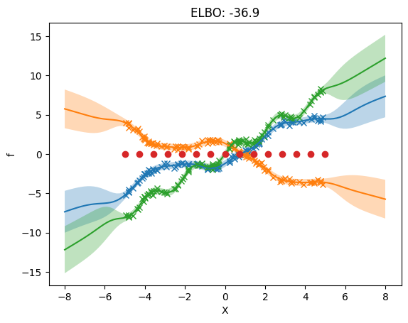
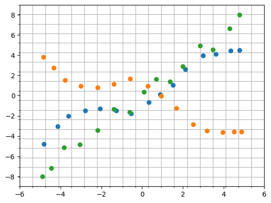
../../_images/notebooks_advanced_multioutput_29_0.png

The following plot shows that we use different inducing inputs in each output dimension.

[22]:

for i in range(len(m.inducing_variable.inducing_variable_list)):
    q_mu_unwhitened, q_var_unwhitened = m.predict_f(
        m.inducing_variable.inducing_variable_list[i].Z
    )
    plt.plot(
        m.inducing_variable.inducing_variable_list[i].Z.numpy(),
        q_mu_unwhitened[:, i, None].numpy(),
        "o",
    )
plt.gca().set_xticks(np.linspace(-6, 6, 20), minor=True)
plt.gca().set_yticks(np.linspace(-9, 9, 20), minor=True)
plt.grid(which="minor")

../../_images/notebooks_advanced_multioutput_31_0.png

[23]:

m.inducing_variable.inducing_variable_list

[23]:

ListWrapper([<gpflow.inducing_variables.inducing_variables.InducingPoints object at 0x7f4b08882bd0>, <gpflow.inducing_variables.inducing_variables.InducingPoints object at 0x7f4b09922710>, <gpflow.inducing_variables.inducing_variables.InducingPoints object at 0x7f4b0418af50>])

Model \(f(x)\) by doing inference in the \(g\) space#

Mixed kernel and uncorrelated inducing variables#

Remember the general case: \(f(x) = W g(x)\), where \(g(x) \in \mathbb{R}^L\), \(f(x) \in \mathbb{R}^P\) and \(W \in \mathbb{R}^{P \times L}\), where \(L \leq P\). We assume that the outputs of \(g\) are uncorrelated, and by mixing them with \(W\) they become correlated. With this setup we perform the optimal routine to calculate the conditional. Namely, calculate the conditional of the uncorrelated latent \(g\) and afterwards project the mean and variance using the mixing matrix: \(\mu_f = W \mu_g\) and \(\Sigma_f = W\Sigma_g W^\top\)

\(K_{uu} = L \times M \times M\)
\(K_{uf} = L \times M \times N\)

[24]:

# Create list of kernels for each output
kern_list = [
    gpf.kernels.SquaredExponential() + gpf.kernels.Linear() for _ in range(L)
]
# Create multi-output kernel from kernel list
kernel = gpf.kernels.LinearCoregionalization(
    kern_list, W=np.random.randn(P, L)
)  # Notice that we initialise the mixing matrix W
# initialisation of inducing input locations (M random points from the training inputs)
Z = Zinit.copy()
# create multi-output inducing variables from Z
iv = gpf.inducing_variables.SharedIndependentInducingVariables(
    gpf.inducing_variables.InducingPoints(Z)
)

[25]:

# initialize mean of variational posterior to be of shape MxL
q_mu = np.zeros((M, L))
# initialize \sqrt(Σ) of variational posterior to be of shape LxMxM
q_sqrt = np.repeat(np.eye(M)[None, ...], L, axis=0) * 1.0

# create SVGP model as usual and optimize
m = gpf.models.SVGP(
    kernel,
    gpf.likelihoods.Gaussian(),
    inducing_variable=iv,
    q_mu=q_mu,
    q_sqrt=q_sqrt,
)

[26]:

optimize_model_with_scipy(m)

 This problem is unconstrained.

RUNNING THE L-BFGS-B CODE

           * * *

Machine precision = 2.220D-16
 N =          298     M =           10

At X0         0 variables are exactly at the bounds

At iterate    0    f=  7.44521D+03    |proj g|=  6.62929D+03


At iterate   50    f=  3.17536D+02    |proj g|=  4.85678D+00


At iterate  100    f=  1.71814D+02    |proj g|=  1.35957D+02

At iterate  150    f=  1.03408D+02    |proj g|=  1.54598D+02


At iterate  200    f=  3.33945D+01    |proj g|=  3.82713D+01

At iterate  250    f=  2.13996D+01    |proj g|=  5.37833D+01


At iterate  300    f=  1.71520D+01    |proj g|=  2.73838D+01

At iterate  350    f=  1.27657D+01    |proj g|=  3.25960D+01


At iterate  400    f=  9.67997D+00    |proj g|=  2.69073D+01

At iterate  450    f=  7.61284D+00    |proj g|=  7.31885D+00


At iterate  500    f=  6.06674D+00    |proj g|=  1.91774D+01

At iterate  550    f=  4.97226D+00    |proj g|=  1.47615D+01


At iterate  600    f=  4.14799D+00    |proj g|=  6.00751D+00

At iterate  650    f=  3.48993D+00    |proj g|=  1.04231D+01


At iterate  700    f=  3.04828D+00    |proj g|=  1.67168D+01

At iterate  750    f=  2.72907D+00    |proj g|=  7.23828D+00


At iterate  800    f=  2.41559D+00    |proj g|=  1.15389D+01

At iterate  850    f=  1.83715D+00    |proj g|=  4.61493D+00


At iterate  900    f=  1.54304D+00    |proj g|=  4.22855D+00

At iterate  950    f=  1.29959D+00    |proj g|=  1.24710D+00


At iterate 1000    f=  1.18640D+00    |proj g|=  3.04028D+00

At iterate 1050    f=  1.08129D+00    |proj g|=  6.13046D+00


At iterate 1100    f=  1.00477D+00    |proj g|=  2.43149D+00

At iterate 1150    f=  9.25643D-01    |proj g|=  6.75472D+00


At iterate 1200    f=  8.69783D-01    |proj g|=  1.66657D+00

At iterate 1250    f=  8.39237D-01    |proj g|=  6.91428D-01


At iterate 1300    f=  8.10740D-01    |proj g|=  6.57386D+00

At iterate 1350    f=  7.83474D-01    |proj g|=  7.78541D-01


At iterate 1400    f=  7.58686D-01    |proj g|=  7.30850D-01

At iterate 1450    f=  7.31603D-01    |proj g|=  1.15340D+00


At iterate 1500    f=  7.11659D-01    |proj g|=  8.92315D-01

At iterate 1550    f=  6.96505D-01    |proj g|=  1.35317D+00


At iterate 1600    f=  6.82715D-01    |proj g|=  1.33298D+00

At iterate 1650    f=  6.71177D-01    |proj g|=  3.28119D+00


At iterate 1700    f=  6.59102D-01    |proj g|=  5.51186D-01

At iterate 1750    f=  6.49904D-01    |proj g|=  6.18087D-01


At iterate 1800    f=  6.41539D-01    |proj g|=  2.11187D-01

At iterate 1850    f=  6.36751D-01    |proj g|=  9.81126D-01


At iterate 1900    f=  6.31310D-01    |proj g|=  1.02064D+00

At iterate 1950    f=  6.24591D-01    |proj g|=  5.50752D-01


At iterate 2000    f=  6.20926D-01    |proj g|=  3.24211D-01

           * * *

Tit   = total number of iterations
Tnf   = total number of function evaluations
Tnint = total number of segments explored during Cauchy searches
Skip  = number of BFGS updates skipped
Nact  = number of active bounds at final generalized Cauchy point
Projg = norm of the final projected gradient
F     = final function value

           * * *

   N    Tit     Tnf  Tnint  Skip  Nact     Projg        F
  298   2000   2182      1     0     0   3.242D-01   6.209D-01
  F =  0.62092649212238626

STOP: TOTAL NO. of ITERATIONS REACHED LIMIT

[27]:

plot_model(m)

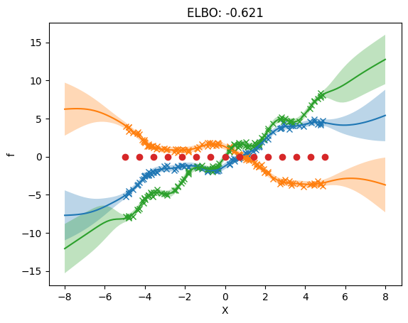
../../_images/notebooks_advanced_multioutput_37_0.png

Illustration of GPflow’s multi-output capabilities#

This section shows the inheritance structure in GPflow’s multi-output framework.

Multi-output kernels (MOK) class diagram#

We include three multi-output kernels: - SharedIndependent: This kernel is included mainly as an illustration of specifying a conditional using the multiple dispatch framework. The same functionality is provided by using a normal kernel and passing in multiple approximate posteriors by stacking q_mu and q_sqrt. - SeparateIndependent: This kernel allows you to use different priors for each output GP. - LinearCoregionalization: This kernel describes the prior of the linear model of coregionalization. As shown previously, this implementation supports various inducing point approximations. Multi-output kernels

We include several base classes. Two are noteworthy: - MultioutputKernel is included to be the base class for all multi-output kernels. - IndepedentLatent is the base class for all multi-output kernels which are constructed from independent latent processes. Including this kernel allows the specification of a default approximation method which, while not the most efficient, does take advantage of some structure. It can be applied to any kernel constructed from independent latent processes.

There is a similarity in the meaning of SeparateIndependent and IndependentLatent. Both kernels indicate that independent processes are used, and that \(\mathbf{K}_{\bf uu}\) can therefore be represented as a [L, M, M] tensor. It could therefore be suggested that SeparateIndependent be the parent class of all “independent latent” kernels, instead of having a separate IndependentLatent class. We decided against this because: - this would increase the complexity in specifying conditionals() for the otherwise simple multi-output kernels SeparateIndependent and SharedIndependent. - we did not want to specify too much of an implementation in IndependentLatent, leaving implementation details to child classes. Using SeparateIndependent as the base class would force all child classes to be a Combination kernel.

Multi-output inducing variables class diagram#

Multi-output features

Inducing points#

The goal of this class is to provide inducing variables that can be used with any kernel, even if the method ends up being slow.

The multiouput framework extends InducingPoints to work with multi-output kernels. Just like for single-output kernels, we want InducingPoints to work for all MultioutputKernels. We do this by defining InducingPoints to take all outputs for specific inducing inputs as inducing variables.

Fallback shared/separate independent inducing variables#

The goal of these classes is to provide a reasonably efficient implementation for kernels that give exploitable independence structure in the prior of inducing variables (that is, subclasses of IndependentLatent), while only needing to implement Kuu() and Kuf() methods.

Shared/separate independent inducing variables#

The goal of these classes is to provide the most efficient code path for kernels that allow exploiting independence structure in the prior of inducing variables.

For more specialized multi-output kernels (i.e. {Shared|Separate}Independent or LinearCoregionalization) we define {Shared|Separate}IndependentInducingVariables. These wrap (a list of) single-output inducing variables to define groups of a-priori independent inducing variables, which leads to a \(\mathbf{K}_{\bf uu}\) that can be represented as a [L, M, M] tensor. We saw the use of these previously.

{Shared|Separate}IndependentInducingVariables inherit from Fallback{Shared|Separate}IndependentInducingVariables, so the multiple dispatch will fall back on the slower but general implementation.

Implemented combinations#

Multiple dispatch is applied to both Kuu(), Kuf(), and conditional(). The return values of the covariances can therefore be tailored to a specific implementation of conditional(). The following table lists combinations which are currently available in GPflow. Thanks to the multiple dispatch code, implementing your own outside of GPflow should require only a small amount of code!

Inducing variable class	Kernel	Kuu	Kuf	conditional	note
`InducingPoints`	`MultioutputKernel`	`[M, P, M, P]`	`[M, P, N, P]`	`inducing_point_conditional()`, which calls `fully_correlated_conditional()`	Works for all kernels, but might be very inefficient. In this case `q_mu` and `q_sqrt` should have shapes of `[1, MP]` and `[1, MP, MP]`
`SharedIndependentInducingVariables`	`SharedIndependent`	`[M, M]`	`[M, N]`	`shared_independent_conditional()`, which calls `base_conditional()`	The combination of these two classes is in a sense redundant, because we can achieve the same behavior by using the single output Kernel and InducingVariable classes. They are added for illustrative purposes. Thanks to the conditional dispatch, the most efficient code path is used.
`SeparateIndependentInducingVariables`	`SharedIndependent`	`[P, M, M]`	`[P, M, N]`	`separate_independent_conditional()`, which calls `base_conditional()` P times	We loop P times over the `base_conditional()`
`SeparateIndependentInducingVariable`	`SeparateIndependent`	`[P, M, M]`	`[P, M, N]`	`separate_independent_conditional()`, which calls `base_conditional()` P times	We loop P times over the `base_conditional()`
`SharedIndependentInducingVariables`	`SeparateIndependent`	`[P, M, M]`	`[P, M, N]`	`separate_independent_conditional()`, which calls `base_conditional()` P times	We loop P times over the `base_conditional()`
`FallbackSharedIndependentInducingVariables`	`IndependentLatent`	`[L, M, M]`	`[M, L, N, P]`	`fallback_independent_latent_conditional()`, which calls `independent_interdomain_conditional()`	Implementation which only requires custom `Kuu()` and `Kuf()`
`FallbackSeparateIndependentInducingVariable`	`IndependentLatent`	`[L, M, M]`	`[M, L, N, P]`	`fallback_independent_latent_conditional()`, which calls `independent_interdomain_conditional()`	Implementation which only requires custom `Kuu()` and `Kuf()`
`SharedIndependentInducingVariables`	`LinearCoregionalization`	`[L, M, M]`	`[L, M, N]`	`coregionalization_conditional()`, which calls `base_conditional()`	This is the most efficient implementation for linear coregionalization. The inducing outputs live in g-space. Here we use the output of the base conditional and project the mean and covariance with the mixing matrix W.
`SeparateIndependentInducingVariables`	`LinearCoregionalization`	`[L, M, M]`	`[L, M, N]`	`base_conditional()`	This is the most efficient implementation for linear coregionalization. The inducing outputs live in g-space. Here we use the output of the base conditional and project the mean and covariance with the mixing matrix W.

Debugging: introspect#

Given all these possibilities it can be hard to determine which conditional will be called for which set of kernel and inducing variable. The following method lets you proactively introspect which implementation will be executed. This can be useful when debugging new code.

[28]:

def inspect_conditional(inducing_variable_type, kernel_type):
    """
    Helper function returning the exact implementation called
    by the multiple dispatch `conditional` given the type of
    kernel and inducing variable.

    :param inducing_variable_type:
        Type of the inducing variable
    :param kernel_type:
        Type of the kernel

    :return: String
        Contains the name, the file and the linenumber of the
        implementation.
    """
    import inspect

    from gpflow.conditionals import conditional

    implementation = conditional.dispatch(
        object, inducing_variable_type, kernel_type, object
    )
    info = dict(inspect.getmembers(implementation))
    return info["__code__"]


# Example:
inspect_conditional(
    gpf.inducing_variables.SharedIndependentInducingVariables,
    gpf.kernels.SharedIndependent,
)

[28]:

<code object wrapped_function at 0x561e2e22a830, file "/tmp/max_venv/lib/python3.11/site-packages/check_shapes/decorator.py", line 120>