Bayesian Gaussian process latent variable model (Bayesian GPLVM)

This notebook shows how to use the Bayesian GPLVM model. This is an unsupervised learning method usually used for dimensionality reduction. For an in-depth overview of GPLVMs,see [1, 2].

import matplotlib.pyplot as plt
import numpy as np
import tensorflow as tf

import gpflow
from gpflow.ci_utils import reduce_in_tests
from gpflow.config import (
    default_float,
    set_default_float,
    set_default_summary_fmt,
)
from gpflow.utilities import ops, print_summary

set_default_float(np.float64)
set_default_summary_fmt("notebook")

%matplotlib inline

2024-02-07 11:46:04.876362: I external/local_tsl/tsl/cuda/cudart_stub.cc:31] Could not find cuda drivers on your machine, GPU will not be used.
2024-02-07 11:46:04.917803: E external/local_xla/xla/stream_executor/cuda/cuda_dnn.cc:9261] Unable to register cuDNN factory: Attempting to register factory for plugin cuDNN when one has already been registered
2024-02-07 11:46:04.917838: E external/local_xla/xla/stream_executor/cuda/cuda_fft.cc:607] Unable to register cuFFT factory: Attempting to register factory for plugin cuFFT when one has already been registered
2024-02-07 11:46:04.919255: E external/local_xla/xla/stream_executor/cuda/cuda_blas.cc:1515] Unable to register cuBLAS factory: Attempting to register factory for plugin cuBLAS when one has already been registered
2024-02-07 11:46:04.926149: I external/local_tsl/tsl/cuda/cudart_stub.cc:31] Could not find cuda drivers on your machine, GPU will not be used.
2024-02-07 11:46:04.926680: I tensorflow/core/platform/cpu_feature_guard.cc:182] This TensorFlow binary is optimized to use available CPU instructions in performance-critical operations.
To enable the following instructions: AVX2 AVX512F FMA, in other operations, rebuild TensorFlow with the appropriate compiler flags.

2024-02-07 11:46:06.009886: W tensorflow/compiler/tf2tensorrt/utils/py_utils.cc:38] TF-TRT Warning: Could not find TensorRT

Data

We are using the “three phase oil flow” dataset used initially for demonstrating the Generative Topographic mapping from [3].

data = np.load("./data/three_phase_oil_flow.npz")

Following the GPflow notation we assume this dataset has a shape of [num_data, output_dim]

Y = tf.convert_to_tensor(data["Y"], dtype=default_float())

Integer in \([0, 2]\) indicating to which class the data point belongs (shape [num_data,]). Not used for model fitting, only for plotting afterwards.

labels = tf.convert_to_tensor(data["labels"])

print(
    "Number of points: {} and Number of dimensions: {}".format(
        Y.shape[0], Y.shape[1]
    )
)

Number of points: 100 and Number of dimensions: 12

Model construction

We start by initializing the required variables:

latent_dim = 2  # number of latent dimensions
num_inducing = 20  # number of inducing pts
num_data = Y.shape[0]  # number of data points

Initialize via PCA:

X_mean_init = ops.pca_reduce(Y, latent_dim)
X_var_init = tf.ones((num_data, latent_dim), dtype=default_float())

Pick inducing inputs randomly from dataset initialization:

np.random.seed(1)  # for reproducibility
inducing_variable = tf.convert_to_tensor(
    np.random.permutation(X_mean_init.numpy())[:num_inducing],
    dtype=default_float(),
)

We construct a Squared Exponential (SE) kernel operating on the two-dimensional latent space. The ARD parameter stands for Automatic Relevance Determination, which in practice means that we learn a different lengthscale for each of the input dimensions. See Manipulating kernels for more information.

lengthscales = tf.convert_to_tensor([1.0] * latent_dim, dtype=default_float())
kernel = gpflow.kernels.RBF(lengthscales=lengthscales)

We have all the necessary ingredients to construct the model. GPflow contains an implementation of the Bayesian GPLVM:

gplvm = gpflow.models.BayesianGPLVM(
    Y,
    X_data_mean=X_mean_init,
    X_data_var=X_var_init,
    kernel=kernel,
    inducing_variable=inducing_variable,
)
# Instead of passing an inducing_variable directly, we can also set the num_inducing_variables argument to an integer, which will randomly pick from the data.

We change the default likelihood variance, which is 1, to 0.01.

gplvm.likelihood.variance.assign(0.01)

<tf.Variable 'UnreadVariable' shape=() dtype=float64, numpy=-4.600266525158521>

Next we optimize the created model. Given that this model has a deterministic evidence lower bound (ELBO), we can use SciPy’s BFGS optimizer.

opt = gpflow.optimizers.Scipy()
maxiter = reduce_in_tests(1000)
opt.minimize(
    gplvm.training_loss,
    method="BFGS",
    variables=gplvm.trainable_variables,
    options=dict(maxiter=maxiter),
)

Model analysis

GPflow allows you to inspect the learned model hyperparameters.

print_summary(gplvm)

name	class	transform	prior	trainable	shape	dtype	value
BayesianGPLVM.kernel.variance	Parameter	Softplus		True	()	float64	0.9180110289150046
BayesianGPLVM.kernel.lengthscales	Parameter	Softplus		True	(2,)	float64	[0.86661109 1.76001 ]
BayesianGPLVM.likelihood.variance	Parameter	Softplus + Shift		True	()	float64	0.006477223077400491
BayesianGPLVM.X_data_mean	Parameter	Identity		True	(100, 2)	float64	[[-7.98779573e-01, 3.04430000e+00...
BayesianGPLVM.X_data_var	Parameter	Softplus		True	(100, 2)	float64	[[0.00040637, 0.00153665...
BayesianGPLVM.inducing_variable.Z	Parameter	Identity		True	(20, 2)	float64	[[1.31767000e+00, -1.72367000e+00...

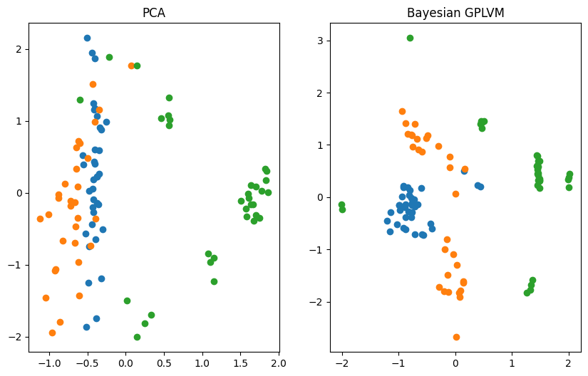
Plotting vs. Principle Component Analysis (PCA)

The reduction of the dimensionality of the dataset to two dimensions allows us to visualize the learned manifold. We compare the Bayesian GPLVM’s latent space to the deterministic PCA’s one.

X_pca = ops.pca_reduce(Y, latent_dim).numpy()
gplvm_X_mean = gplvm.X_data_mean.numpy()

f, ax = plt.subplots(1, 2, figsize=(10, 6))

for i in np.unique(labels):
    ax[0].scatter(X_pca[labels == i, 0], X_pca[labels == i, 1], label=i)
    ax[1].scatter(
        gplvm_X_mean[labels == i, 0], gplvm_X_mean[labels == i, 1], label=i
    )
    ax[0].set_title("PCA")
    ax[1].set_title("Bayesian GPLVM")

References

[1] Lawrence, Neil D. ‘Gaussian process latent variable models for visualization of high dimensional data’. Advances in Neural Information Processing Systems. 2004.

[2] Titsias, Michalis, and Neil D. Lawrence. ‘Bayesian Gaussian process latent variable model’. Proceedings of the Thirteenth International Conference on Artificial Intelligence and Statistics. 2010.

[3] Bishop, Christopher M., and Gwilym D. James. ‘Analysis of multiphase flows using dual-energy gamma densitometry and neural networks’. Nuclear Instruments and Methods in Physics Research Section A: Accelerators, Spectrometers, Detectors and Associated Equipment 327.2-3 (1993): 580-593.