Ordinal regression

Ordinal regression aims to fit a model to some data \((X, Y)\), where \(Y\) is an ordinal variable. To do so, we use a VPG model with a specific likelihood (gpflow.likelihoods.Ordinal).

import matplotlib.pyplot as plt
import numpy as np

import gpflow

%matplotlib inline
plt.rcParams["figure.figsize"] = (12, 6)

np.random.seed(123)  # for reproducibility

2024-02-07 11:46:19.927440: I external/local_tsl/tsl/cuda/cudart_stub.cc:31] Could not find cuda drivers on your machine, GPU will not be used.
2024-02-07 11:46:19.971205: E external/local_xla/xla/stream_executor/cuda/cuda_dnn.cc:9261] Unable to register cuDNN factory: Attempting to register factory for plugin cuDNN when one has already been registered
2024-02-07 11:46:19.971255: E external/local_xla/xla/stream_executor/cuda/cuda_fft.cc:607] Unable to register cuFFT factory: Attempting to register factory for plugin cuFFT when one has already been registered
2024-02-07 11:46:19.972814: E external/local_xla/xla/stream_executor/cuda/cuda_blas.cc:1515] Unable to register cuBLAS factory: Attempting to register factory for plugin cuBLAS when one has already been registered
2024-02-07 11:46:19.980013: I external/local_tsl/tsl/cuda/cudart_stub.cc:31] Could not find cuda drivers on your machine, GPU will not be used.
2024-02-07 11:46:19.980582: I tensorflow/core/platform/cpu_feature_guard.cc:182] This TensorFlow binary is optimized to use available CPU instructions in performance-critical operations.
To enable the following instructions: AVX2 AVX512F FMA, in other operations, rebuild TensorFlow with the appropriate compiler flags.

2024-02-07 11:46:21.123620: W tensorflow/compiler/tf2tensorrt/utils/py_utils.cc:38] TF-TRT Warning: Could not find TensorRT

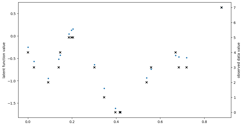
# make a one-dimensional ordinal regression problem

# This function generates a set of inputs X,
# quantitative output f (latent) and ordinal values Y


def generate_data(num_data):
    # First generate random inputs
    X = np.random.rand(num_data, 1)

    # Now generate values of a latent GP
    kern = gpflow.kernels.SquaredExponential(lengthscales=0.1)
    K = kern(X)
    f = np.random.multivariate_normal(mean=np.zeros(num_data), cov=K).reshape(
        -1, 1
    )

    # Finally convert f values into ordinal values Y
    Y = np.round((f + f.min()) * 3)
    Y = Y - Y.min()
    Y = np.asarray(Y, np.float64)

    return X, f, Y


np.random.seed(1)
num_data = 20
X, f, Y = generate_data(num_data)

plt.figure(figsize=(11, 6))
plt.plot(X, f, ".")
plt.ylabel("latent function value")

plt.twinx()
plt.plot(X, Y, "kx", mew=1.5)
plt.ylabel("observed data value")

Text(0, 0.5, 'observed data value')

# construct ordinal likelihood - bin_edges is the same as unique(Y) but centered
bin_edges = np.array(np.arange(np.unique(Y).size + 1), dtype=float)
bin_edges = bin_edges - bin_edges.mean()
likelihood = gpflow.likelihoods.Ordinal(bin_edges)

# build a model with this likelihood
m = gpflow.models.VGP(
    data=(X, Y), kernel=gpflow.kernels.Matern32(), likelihood=likelihood
)

# fit the model
opt = gpflow.optimizers.Scipy()
opt.minimize(m.training_loss, m.trainable_variables, options=dict(maxiter=100))

  message: STOP: TOTAL NO. of ITERATIONS REACHED LIMIT
  success: False
   status: 1
      fun: 25.487473214735196
        x: [-2.000e+00 -2.362e-01 ...  5.467e+00 -1.450e+00]
      nit: 100
      jac: [-6.701e-02 -2.637e-02 ... -8.499e-03 -9.853e-03]
     nfev: 116
     njev: 116
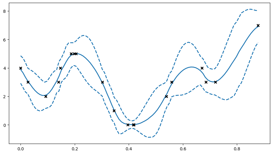
 hess_inv: <233x233 LbfgsInvHessProduct with dtype=float64>

# here we'll plot the expected value of Y +- 2 std deviations, as if the distribution were Gaussian
plt.figure(figsize=(11, 6))
X_data, Y_data = (m.data[0].numpy(), m.data[1].numpy())
Xtest = np.linspace(X_data.min(), X_data.max(), 100).reshape(-1, 1)
mu, var = m.predict_y(Xtest)
(line,) = plt.plot(Xtest, mu, lw=2)
col = line.get_color()
plt.plot(Xtest, mu + 2 * np.sqrt(var), "--", lw=2, color=col)
plt.plot(Xtest, mu - 2 * np.sqrt(var), "--", lw=2, color=col)
plt.plot(X_data, Y_data, "kx", mew=2)

[<matplotlib.lines.Line2D at 0x7f4fe1761990>]

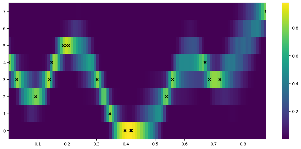
## to see the predictive density, try predicting every possible discrete value for Y.
def pred_log_density(m):
    Xtest = np.linspace(X_data.min(), X_data.max(), 100).reshape(-1, 1)
    ys = np.arange(Y_data.max() + 1)
    densities = []
    for y in ys:
        Ytest = np.full_like(Xtest, y)
        # Predict the log density
        densities.append(m.predict_log_density((Xtest, Ytest)))
    return np.vstack(densities)

fig = plt.figure(figsize=(14, 6))
plt.imshow(
    np.exp(pred_log_density(m)),
    interpolation="nearest",
    extent=[X_data.min(), X_data.max(), -0.5, Y_data.max() + 0.5],
    origin="lower",
    aspect="auto",
    cmap=plt.cm.viridis,
)
plt.colorbar()
plt.plot(X, Y, "kx", mew=2, scalex=False, scaley=False)

[<matplotlib.lines.Line2D at 0x7f4fe1698450>]

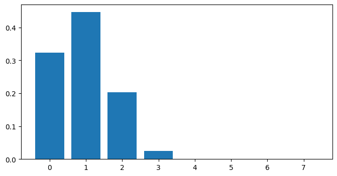
# Predictive density for a single input x=0.5
x_new = 0.5
Y_new = np.arange(np.max(Y_data + 1)).reshape([-1, 1])
X_new = np.full_like(Y_new, x_new)
# for predict_log_density x and y need to have the same number of rows
dens_new = np.exp(m.predict_log_density((X_new, Y_new)))
fig = plt.figure(figsize=(8, 4))
plt.bar(x=Y_new.flatten(), height=dens_new.flatten())

<BarContainer object of 8 artists>