Comparing FITC approximation to VFE approximation

This notebook examines why we prefer the Variational Free Energy (VFE) objective to the Fully Independent Training Conditional (FITC) approximation for our sparse approximations.

import matplotlib.pyplot as plt
from FITCvsVFE import (
    getTrainingTestData,
    plotComparisonFigure,
    plotPredictions,
    printModelParameters,
    repeatMinimization,
    stretch,
)

import gpflow
from gpflow.ci_utils import reduce_in_tests

%matplotlib inline


# logging.disable(logging.WARN)  # do not clutter up the notebook with optimization warnings

2024-02-07 11:47:07.707919: I external/local_tsl/tsl/cuda/cudart_stub.cc:31] Could not find cuda drivers on your machine, GPU will not be used.
2024-02-07 11:47:07.750453: E external/local_xla/xla/stream_executor/cuda/cuda_dnn.cc:9261] Unable to register cuDNN factory: Attempting to register factory for plugin cuDNN when one has already been registered
2024-02-07 11:47:07.750499: E external/local_xla/xla/stream_executor/cuda/cuda_fft.cc:607] Unable to register cuFFT factory: Attempting to register factory for plugin cuFFT when one has already been registered
2024-02-07 11:47:07.752074: E external/local_xla/xla/stream_executor/cuda/cuda_blas.cc:1515] Unable to register cuBLAS factory: Attempting to register factory for plugin cuBLAS when one has already been registered
2024-02-07 11:47:07.758790: I external/local_tsl/tsl/cuda/cudart_stub.cc:31] Could not find cuda drivers on your machine, GPU will not be used.
2024-02-07 11:47:07.759367: I tensorflow/core/platform/cpu_feature_guard.cc:182] This TensorFlow binary is optimized to use available CPU instructions in performance-critical operations.
To enable the following instructions: AVX2 AVX512F FMA, in other operations, rebuild TensorFlow with the appropriate compiler flags.

2024-02-07 11:47:08.806954: W tensorflow/compiler/tf2tensorrt/utils/py_utils.cc:38] TF-TRT Warning: Could not find TensorRT

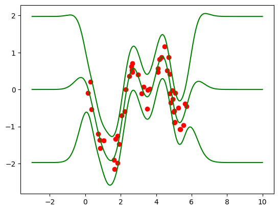
First, we load the training data and plot it together with the exact GP solution (using the GPR model):

# Load the training data:
Xtrain, Ytrain, Xtest, Ytest = getTrainingTestData()


def getKernel():
    return gpflow.kernels.SquaredExponential()


# Run exact inference on training data:
exact_model = gpflow.models.GPR((Xtrain, Ytrain), kernel=getKernel())

opt = gpflow.optimizers.Scipy()
opt.minimize(
    exact_model.training_loss,
    exact_model.trainable_variables,
    method="L-BFGS-B",
    options=dict(maxiter=reduce_in_tests(20000)),
    tol=1e-11,
)

print("Exact model parameters:")
printModelParameters(exact_model)

figA, ax = plt.subplots(1, 1)
ax.plot(Xtrain, Ytrain, "ro")
plotPredictions(ax, exact_model, color="g")

Exact model parameters:
  Likelihood variance = 0.074285
  Kernel variance     = 0.90049
  Kernel lengthscale  = 0.5825

def initializeHyperparametersFromExactSolution(sparse_model):
    sparse_model.likelihood.variance.assign(exact_model.likelihood.variance)
    sparse_model.kernel.variance.assign(exact_model.kernel.variance)
    sparse_model.kernel.lengthscales.assign(exact_model.kernel.lengthscales)

We now construct two sparse model using the VFE (SGPR model) and FITC (GPRFITC model) optimization objectives, with the inducing points being initialized on top of the training inputs, and the model hyperparameters (kernel variance and lengthscales, and likelihood variance) being initialized to the values obtained in the optimization of the exact GPR model:

# Train VFE model initialized from the perfect solution.
VFEmodel = gpflow.models.SGPR(
    (Xtrain, Ytrain), kernel=getKernel(), inducing_variable=Xtrain.copy()
)

initializeHyperparametersFromExactSolution(VFEmodel)

VFEcb = repeatMinimization(
    VFEmodel, Xtest, Ytest
)  # optimize with several restarts
print("Sparse model parameters after VFE optimization:")
printModelParameters(VFEmodel)

Sparse model parameters after VFE optimization:
  Likelihood variance = 0.074286
  Kernel variance     = 0.90049
  Kernel lengthscale  = 0.5825

# Train FITC model initialized from the perfect solution.
FITCmodel = gpflow.models.GPRFITC(
    (Xtrain, Ytrain), kernel=getKernel(), inducing_variable=Xtrain.copy()
)

initializeHyperparametersFromExactSolution(FITCmodel)

FITCcb = repeatMinimization(
    FITCmodel, Xtest, Ytest
)  # optimize with several restarts
print("Sparse model parameters after FITC optimization:")
printModelParameters(FITCmodel)

Sparse model parameters after FITC optimization:
  Likelihood variance = 0.01898
  Kernel variance     = 1.3328
  Kernel lengthscale  = 0.61755

Plotting a comparison of the two algorithms, we see that VFE stays at the optimum of exact GPR, whereas the FITC approximation eventually ends up with several inducing points on top of each other, and a worse fit:

figB, axes = plt.subplots(3, 2, figsize=(20, 16))

# VFE optimization finishes after 10 iterations, so we stretch out the training and test
# log-likelihood traces to make them comparable against FITC:
VFEiters = FITCcb.n_iters
VFElog_likelihoods = stretch(len(VFEiters), VFEcb.log_likelihoods)
VFEhold_out_likelihood = stretch(len(VFEiters), VFEcb.hold_out_likelihood)

axes[0, 0].set_title("VFE", loc="center", fontdict={"fontsize": 22})
plotComparisonFigure(
    Xtrain,
    VFEmodel,
    exact_model,
    axes[0, 0],
    axes[1, 0],
    axes[2, 0],
    VFEiters,
    VFElog_likelihoods,
    VFEhold_out_likelihood,
)

axes[0, 1].set_title("FITC", loc="center", fontdict={"fontsize": 22})
plotComparisonFigure(
    Xtrain,
    FITCmodel,
    exact_model,
    axes[0, 1],
    axes[1, 1],
    axes[2, 1],
    FITCcb.n_iters,
    FITCcb.log_likelihoods,
    FITCcb.hold_out_likelihood,
)

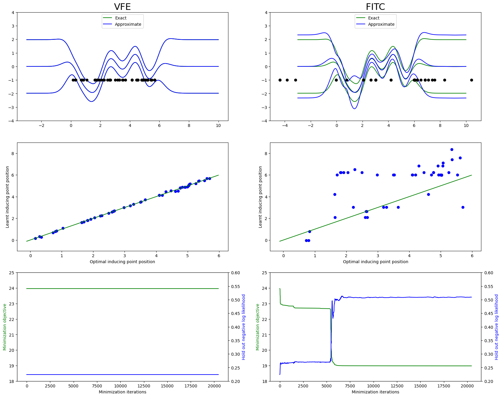
A more detailed discussion of the comparison between these sparse approximations can be found in Understanding Probabilistic Sparse Gaussian Process Approximations by Bauer, van der Wilk, and Rasmussen (2017).