Heteroskedastic Likelihood and Multi-Latent GP

Standard (Homoskedastic) Regression

In standard GP regression, the GP latent function is used to learn the location parameter of a likelihood distribution (usually a Gaussian) as a function of the input \(x\), whereas the scale parameter is considered constant. This is a homoskedastic model, which is unable to capture variations of the noise distribution with the input \(x\).

Heteroskedastic Regression

This notebooks shows how to construct a model which uses multiple (here two) GP latent functions to learn both the location and the scale of the Gaussian likelihood distribution. It does so by connecting a Multi-Output Kernel, which generates multiple GP latent functions, to a Heteroskedastic Likelihood, which maps the latent GPs into a single likelihood.

The generative model is described as:

\[f_1(x) \sim \mathcal{GP}(0, k_1(\cdot, \cdot))\]

\[f_2(x) \sim \mathcal{GP}(0, k_2(\cdot, \cdot))\]

\[\text{loc}(x) = f_1(x)\]

\[\text{scale}(x) = \text{transform}(f_2(x))\]

\[y_i|f_1, f_2, x_i \sim \mathcal{N}(\text{loc}(x_i),\;\text{scale}(x_i)^2)\]

The function \(\text{transform}\) is used to map from the unconstrained GP \(f_2\) to positive-only values, which is required as it represents the \(\text{scale}\) of a Gaussian likelihood. In this notebook, the \(\exp\) function will be used as the \(\text{transform}\). Other positive transforms such as the \(\text{softplus}\) function can also be used.

import matplotlib.pyplot as plt
import numpy as np
import tensorflow as tf
import tensorflow_probability as tfp

import gpflow as gpf

2024-02-07 11:45:59.389733: I external/local_tsl/tsl/cuda/cudart_stub.cc:31] Could not find cuda drivers on your machine, GPU will not be used.
2024-02-07 11:45:59.434481: E external/local_xla/xla/stream_executor/cuda/cuda_dnn.cc:9261] Unable to register cuDNN factory: Attempting to register factory for plugin cuDNN when one has already been registered
2024-02-07 11:45:59.434526: E external/local_xla/xla/stream_executor/cuda/cuda_fft.cc:607] Unable to register cuFFT factory: Attempting to register factory for plugin cuFFT when one has already been registered
2024-02-07 11:45:59.435763: E external/local_xla/xla/stream_executor/cuda/cuda_blas.cc:1515] Unable to register cuBLAS factory: Attempting to register factory for plugin cuBLAS when one has already been registered
2024-02-07 11:45:59.443082: I external/local_tsl/tsl/cuda/cudart_stub.cc:31] Could not find cuda drivers on your machine, GPU will not be used.
2024-02-07 11:45:59.443721: I tensorflow/core/platform/cpu_feature_guard.cc:182] This TensorFlow binary is optimized to use available CPU instructions in performance-critical operations.
To enable the following instructions: AVX2 AVX512F FMA, in other operations, rebuild TensorFlow with the appropriate compiler flags.

2024-02-07 11:46:00.604760: W tensorflow/compiler/tf2tensorrt/utils/py_utils.cc:38] TF-TRT Warning: Could not find TensorRT

Data Generation

We generate heteroskedastic data by substituting the random latent functions \(f_1\) and \(f_2\) of the generative model by deterministic \(\sin\) and \(\cos\) functions. The input \(X\) is built with \(N=1001\) uniformly spaced values in the interval \([0, 4\pi]\). The outputs \(Y\) are still sampled from a Gaussian likelihood.

\[x_i \in [0, 4\pi], \quad i = 1,\dots,N\]

\[f_1(x) = \sin(x)\]

\[f_2(x) = \cos(x)\]

\[\text{loc}(x) = f_1(x)\]

\[\text{scale}(x) = \exp(f_2(x))\]

\[y_i|x_i \sim \mathcal{N}(\text{loc}(x_i),\;\text{scale}(x_i)^2)\]

N = 1001

np.random.seed(0)
tf.random.set_seed(0)

# Build inputs X
X = np.linspace(0, 4 * np.pi, N)[:, None]  # X must be of shape [N, 1]

# Deterministic functions in place of latent ones
f1 = np.sin
f2 = np.cos

# Use transform = exp to ensure positive-only scale values
transform = np.exp

# Compute loc and scale as functions of input X
loc = f1(X)
scale = transform(f2(X))

# Sample outputs Y from Gaussian Likelihood
Y = np.random.normal(loc, scale)

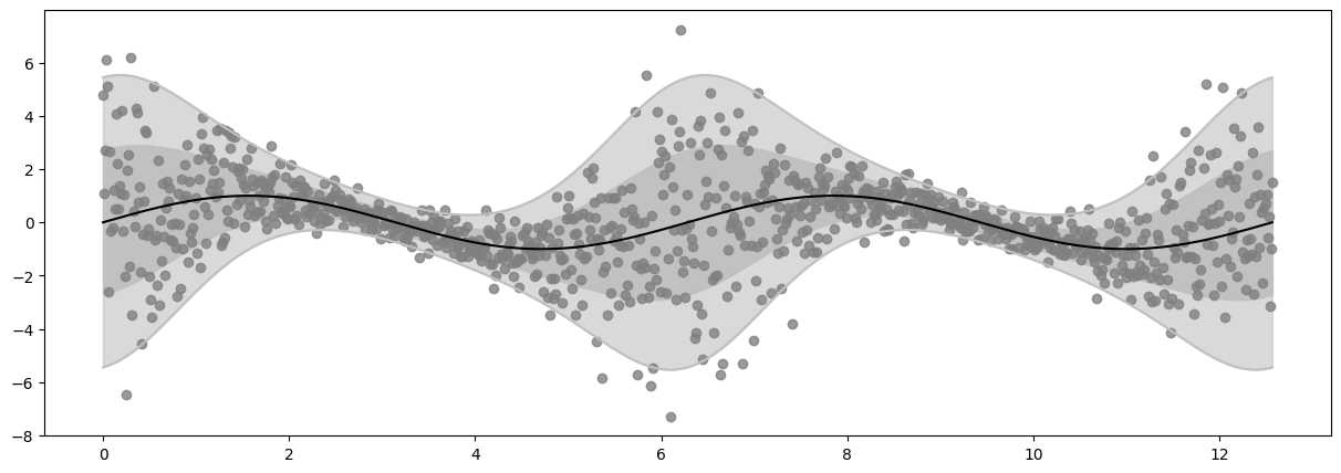
Plot Data

Note how the distribution density (shaded area) and the outputs \(Y\) both change depending on the input \(X\).

def plot_distribution(X, Y, loc, scale):
    plt.figure(figsize=(15, 5))
    x = X.squeeze()
    for k in (1, 2):
        lb = (loc - k * scale).squeeze()
        ub = (loc + k * scale).squeeze()
        plt.fill_between(x, lb, ub, color="silver", alpha=1 - 0.05 * k ** 3)
    plt.plot(x, lb, color="silver")
    plt.plot(x, ub, color="silver")
    plt.plot(X, loc, color="black")
    plt.scatter(X, Y, color="gray", alpha=0.8)
    plt.show()
    plt.close()


plot_distribution(X, Y, loc, scale)

Build Model

Likelihood

This implements the following part of the generative model:

\[\text{loc}(x) = f_1(x)\]

\[\text{scale}(x) = \text{transform}(f_2(x))\]

\[y_i|f_1, f_2, x_i \sim \mathcal{N}(\text{loc}(x_i),\;\text{scale}(x_i)^2)\]

likelihood = gpf.likelihoods.HeteroskedasticTFPConditional(
    distribution_class=tfp.distributions.Normal,  # Gaussian Likelihood
    scale_transform=tfp.bijectors.Exp(),  # Exponential Transform
)

print(f"Likelihood's expected latent_dim: {likelihood.latent_dim}")

Likelihood's expected latent_dim: 2

Kernel

This implements the following part of the generative model:

\[f_1(x) \sim \mathcal{GP}(0, k_1(\cdot, \cdot))\]

\[f_2(x) \sim \mathcal{GP}(0, k_2(\cdot, \cdot))\]

with both kernels being modeled as separate and independent \(\text{SquaredExponential}\) kernels.

kernel = gpf.kernels.SeparateIndependent(
    [
        gpf.kernels.SquaredExponential(),  # This is k1, the kernel of f1
        gpf.kernels.SquaredExponential(),  # this is k2, the kernel of f2
    ]
)
# The number of kernels contained in gpf.kernels.SeparateIndependent must be the same as likelihood.latent_dim

Inducing Points

Since we will use the SVGP model to perform inference, we need to implement the inducing variables \(U_1\) and \(U_2\), both with size \(M=20\), which are used to approximate \(f_1\) and \(f_2\) respectively, and initialize the inducing points positions \(Z_1\) and \(Z_2\). This gives a total of \(2M=40\) inducing variables and inducing points.

The inducing variables and their corresponding inputs will be Separate and Independent, but both \(Z_1\) and \(Z_2\) will be initialized as \(Z\), which are placed as \(M=20\) equally spaced points in \([\min(X), \max(X)]\).

M = 20  # Number of inducing variables for each f_i

# Initial inducing points position Z
Z = np.linspace(X.min(), X.max(), M)[:, None]  # Z must be of shape [M, 1]

inducing_variable = gpf.inducing_variables.SeparateIndependentInducingVariables(
    [
        gpf.inducing_variables.InducingPoints(Z),  # This is U1 = f1(Z1)
        gpf.inducing_variables.InducingPoints(Z),  # This is U2 = f2(Z2)
    ]
)

SVGP Model

Build the SVGP model by composing the Kernel, the Likelihood and the Inducing Variables.

Note that the model needs to be instructed about the number of latent GPs by passing num_latent_gps=likelihood.latent_dim.

model = gpf.models.SVGP(
    kernel=kernel,
    likelihood=likelihood,
    inducing_variable=inducing_variable,
    num_latent_gps=likelihood.latent_dim,
)

model

<gpflow.models.svgp.SVGP object at 0x7efe7c7000d0>

name	class	transform	prior	trainable	shape	dtype	value
SVGP.kernel.kernels[0].variance	Parameter	Softplus		True	()	float64	1.0
SVGP.kernel.kernels[0].lengthscales	Parameter	Softplus		True	()	float64	1.0
SVGP.kernel.kernels[1].variance	Parameter	Softplus		True	()	float64	1.0
SVGP.kernel.kernels[1].lengthscales	Parameter	Softplus		True	()	float64	1.0
SVGP.inducing_variable.inducing_variable_list[0].Z	Parameter	Identity		True	(20, 1)	float64	[[0....
SVGP.inducing_variable.inducing_variable_list[1].Z	Parameter	Identity		True	(20, 1)	float64	[[0....
SVGP.q_mu	Parameter	Identity		True	(20, 2)	float64	[[0., 0....
SVGP.q_sqrt	Parameter	FillTriangular		True	(2, 20, 20)	float64	[[[1., 0., 0....

Model Optimization

Build Optimizers (NatGrad + Adam)

data = (X, Y)
loss_fn = model.training_loss_closure(data)

gpf.utilities.set_trainable(model.q_mu, False)
gpf.utilities.set_trainable(model.q_sqrt, False)

variational_vars = [(model.q_mu, model.q_sqrt)]
natgrad_opt = gpf.optimizers.NaturalGradient(gamma=0.1)

adam_vars = model.trainable_variables
adam_opt = tf.optimizers.Adam(0.01)


@tf.function
def optimisation_step():
    natgrad_opt.minimize(loss_fn, variational_vars)
    adam_opt.minimize(loss_fn, adam_vars)

Run Optimization Loop

epochs = 100
log_freq = 20

for epoch in range(1, epochs + 1):
    optimisation_step()

    # For every 'log_freq' epochs, print the epoch and plot the predictions against the data
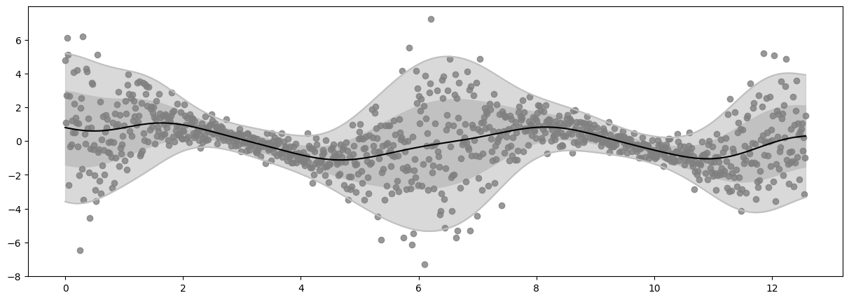
    if epoch % log_freq == 0 and epoch > 0:
        print(f"Epoch {epoch} - Loss: {loss_fn().numpy() : .4f}")
        Ymean, Yvar = model.predict_y(X)
        Ymean = Ymean.numpy().squeeze()
        Ystd = tf.sqrt(Yvar).numpy().squeeze()
        plot_distribution(X, Y, Ymean, Ystd)

model

WARNING:tensorflow:From /tmp/max_venv/lib/python3.11/site-packages/tensorflow/python/util/deprecation.py:660: calling map_fn_v2 (from tensorflow.python.ops.map_fn) with dtype is deprecated and will be removed in a future version.
Instructions for updating:
Use fn_output_signature instead

Epoch 20 - Loss:  1471.8678

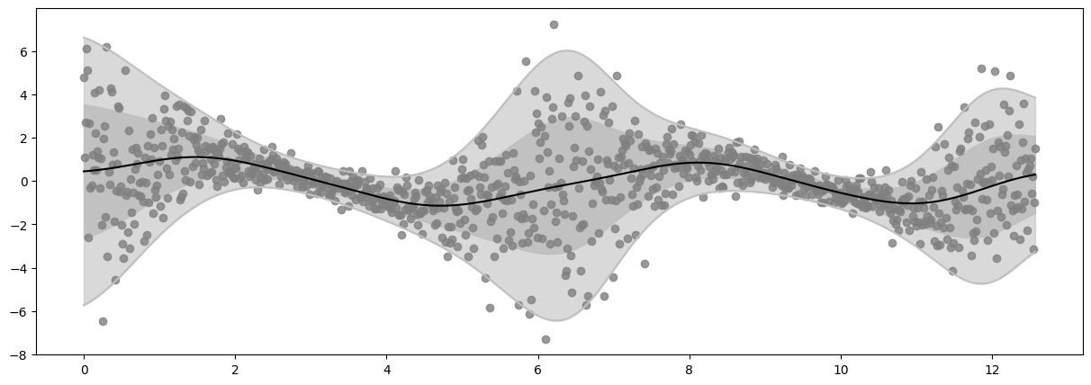
Epoch 40 - Loss:  1452.4426

Epoch 60 - Loss:  1450.7381

Epoch 80 - Loss:  1450.0566

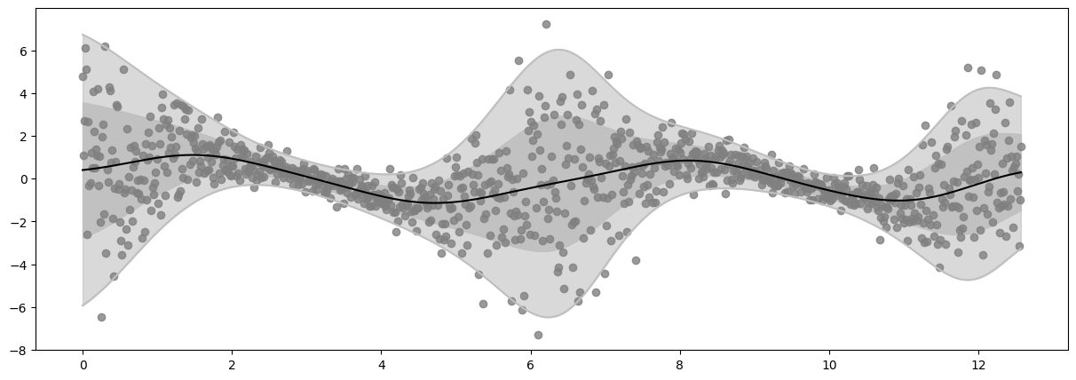
Epoch 100 - Loss:  1449.6073

<gpflow.models.svgp.SVGP object at 0x7efe7c7000d0>

name	class	transform	prior	trainable	shape	dtype	value
SVGP.kernel.kernels[0].variance	Parameter	Softplus		True	()	float64	0.8370710827654084
SVGP.kernel.kernels[0].lengthscales	Parameter	Softplus		True	()	float64	1.18477
SVGP.kernel.kernels[1].variance	Parameter	Softplus		True	()	float64	1.13101
SVGP.kernel.kernels[1].lengthscales	Parameter	Softplus		True	()	float64	1.05985
SVGP.inducing_variable.inducing_variable_list[0].Z	Parameter	Identity		True	(20, 1)	float64	[[-0.1166504...
SVGP.inducing_variable.inducing_variable_list[1].Z	Parameter	Identity		True	(20, 1)	float64	[[-0.2696834...
SVGP.q_mu	Parameter	Identity		False	(20, 2)	float64	[[0.38260668, 1.07056...
SVGP.q_sqrt	Parameter	FillTriangular		False	(2, 20, 20)	float64	[[[4.64009282e-01, 0.00000000e+00, 0.00000000e+00...

Further reading

See Chained Gaussian Processes by Saul et al. (AISTATS 2016).