A simple demonstration of coregionalization

This notebook shows how to construct a multi-output GP model using GPflow. We will consider a regression problem for functions \(f: \mathbb{R}^D \rightarrow \mathbb{R}^P\). We assume that the dataset is of the form \((X_1, f_1), \dots, (X_P, f_P)\), that is, we do not necessarily observe all the outputs for a particular input location (for cases where there are fully observed outputs for each input, see Multi-output Gaussian processes in GPflow for a more efficient implementation). We allow each \(f_i\) to have a different noise distribution by assigning a different likelihood to each.

For this problem, we model \(f\) as a coregionalized Gaussian process, which assumes a kernel of the form:

\begin{equation} \textrm{cov}(f_i(X), f_j(X^\prime)) = k(X, X^\prime) \cdot B[i, j]. \end{equation}

The covariance of the \(i\)th function at \(X\) and the \(j\)th function at \(X^\prime\) is a kernel applied at \(X\) and \(X^\prime\), times the \((i, j)\)th entry of a positive definite \(P \times P\) matrix \(B\). This is known as the intrinsic model of coregionalization (ICM) (Bonilla and Williams, 2008).

To make sure that B is positive-definite, we parameterize it as:

\begin{equation} B = W W^\top + \textrm{diag}(\kappa). \end{equation}

To build such a model in GPflow, we need to perform the following two steps:

• Create the kernel function defined previously, using the Coregion kernel class.

• Augment the training data X with an extra column that contains an integer index to indicate which output an observation is associated with. This is essential to make the data work with the Coregion kernel.

• Create a likelihood for each output using the SwitchedLikelihood class, which is a container for other likelihoods.

• Augment the training data Y with an extra column that contains an integer index to indicate which likelihood an observation is associated with.

import matplotlib.pyplot as plt
import numpy as np

import gpflow
from gpflow.ci_utils import reduce_in_tests

%matplotlib inline

plt.rcParams["figure.figsize"] = (12, 6)
np.random.seed(123)

2024-02-07 11:46:04.119358: I external/local_tsl/tsl/cuda/cudart_stub.cc:31] Could not find cuda drivers on your machine, GPU will not be used.
2024-02-07 11:46:04.165012: E external/local_xla/xla/stream_executor/cuda/cuda_dnn.cc:9261] Unable to register cuDNN factory: Attempting to register factory for plugin cuDNN when one has already been registered
2024-02-07 11:46:04.165053: E external/local_xla/xla/stream_executor/cuda/cuda_fft.cc:607] Unable to register cuFFT factory: Attempting to register factory for plugin cuFFT when one has already been registered
2024-02-07 11:46:04.166436: E external/local_xla/xla/stream_executor/cuda/cuda_blas.cc:1515] Unable to register cuBLAS factory: Attempting to register factory for plugin cuBLAS when one has already been registered
2024-02-07 11:46:04.174039: I external/local_tsl/tsl/cuda/cudart_stub.cc:31] Could not find cuda drivers on your machine, GPU will not be used.
2024-02-07 11:46:04.174932: I tensorflow/core/platform/cpu_feature_guard.cc:182] This TensorFlow binary is optimized to use available CPU instructions in performance-critical operations.
To enable the following instructions: AVX2 AVX512F FMA, in other operations, rebuild TensorFlow with the appropriate compiler flags.

2024-02-07 11:46:05.338645: W tensorflow/compiler/tf2tensorrt/utils/py_utils.cc:38] TF-TRT Warning: Could not find TensorRT

Data preparation

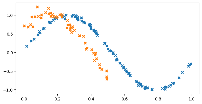
We start by generating some training data to fit the model with. For this example, we choose the following two correlated functions for our outputs:

\begin{align} y_1 &= \sin(6x) + \epsilon_1, \qquad \epsilon_1 \sim \mathcal{N}(0, 0.009) \\ y_2 &= \sin(6x + 0.7) + \epsilon_2, \qquad \epsilon_2 \sim \mathcal{N}(0, 0.01) \end{align}

# make a dataset with two outputs, correlated, heavy-tail noise. One has more noise than the other.
X1 = np.random.rand(100, 1)  # Observed locations for first output
X2 = np.random.rand(50, 1) * 0.5  # Observed locations for second output

Y1 = np.sin(6 * X1) + np.random.randn(*X1.shape) * 0.03
Y2 = np.sin(6 * X2 + 0.7) + np.random.randn(*X2.shape) * 0.1

plt.figure(figsize=(8, 4))
plt.plot(X1, Y1, "x", mew=2)
plt.plot(X2, Y2, "x", mew=2)

Data formatting for the coregionalized model

We add an extra column to our training dataset that contains an index that specifies which output is observed.

# Augment the input with ones or zeros to indicate the required output dimension
X_augmented = np.vstack(
    (np.hstack((X1, np.zeros_like(X1))), np.hstack((X2, np.ones_like(X2))))
)

# Augment the Y data with ones or zeros that specify a likelihood from the list of likelihoods
Y_augmented = np.vstack(
    (np.hstack((Y1, np.zeros_like(Y1))), np.hstack((Y2, np.ones_like(Y2))))
)

Building the coregionalization kernel

We build a coregionalization kernel with the Matern 3/2 kernel as the base kernel. This acts on the leading ([0]) data dimension of the augmented X values. The Coregion kernel indexes the outputs, and acts on the last ([1]) data dimension (indices) of the augmented X values. To specify these dimensions, we use the built-in active_dims argument in the kernel constructor. To construct the full multi-output kernel, we take the product of the two kernels (for a more in-depth tutorial on kernel combination, see Manipulating kernels).

output_dim = 2  # Number of outputs
rank = 1  # Rank of W

# Base kernel
k = gpflow.kernels.Matern32(active_dims=[0])

# Coregion kernel
coreg = gpflow.kernels.Coregion(
    output_dim=output_dim, rank=rank, active_dims=[1]
)

kern = k * coreg

Note: W = 0 is a saddle point in the objective, which would result in the value of W not being optimized to fit the data. Hence, by default, the W matrix is initialized with 0.1. Alternatively, you could re-initialize the matrix to random entries.

Constructing the model

The final element in building the model is to specify the likelihood for each output dimension. To do this, use the SwitchedLikelihood object in GPflow.

# This likelihood switches between Gaussian noise with different variances for each f_i:
lik = gpflow.likelihoods.SwitchedLikelihood(
    [gpflow.likelihoods.Gaussian(), gpflow.likelihoods.Gaussian()]
)

# now build the GP model as normal
m = gpflow.models.VGP((X_augmented, Y_augmented), kernel=kern, likelihood=lik)

# fit the covariance function parameters
maxiter = reduce_in_tests(10000)
gpflow.optimizers.Scipy().minimize(
    m.training_loss,
    m.trainable_variables,
    options=dict(maxiter=maxiter),
    method="L-BFGS-B",
)

  message: CONVERGENCE: REL_REDUCTION_OF_F_<=_FACTR*EPSMCH
  success: True
   status: 0
      fun: -225.66174063752118
        x: [-7.950e-01  2.214e+00 ... -7.390e+00 -4.835e+00]
      nit: 1330
      jac: [ 1.726e-04  1.055e-01 ... -3.278e-03 -4.459e-04]
     nfev: 1455
     njev: 1455
 hess_inv: <11483x11483 LbfgsInvHessProduct with dtype=float64>

That’s it: the model is trained. Let’s plot the model fit to see what’s happened.

def plot_gp(x, mu, var, color, label):
    plt.plot(x, mu, color=color, lw=2, label=label)
    plt.fill_between(
        x[:, 0],
        (mu - 2 * np.sqrt(var))[:, 0],
        (mu + 2 * np.sqrt(var))[:, 0],
        color=color,
        alpha=0.4,
    )


def plot(m):
    plt.figure(figsize=(8, 4))
    Xtest = np.linspace(0, 1, 100)[:, None]
    (line,) = plt.plot(X1, Y1, "x", mew=2)
    mu, var = m.predict_f(np.hstack((Xtest, np.zeros_like(Xtest))))
    plot_gp(Xtest, mu, var, line.get_color(), "Y1")

    (line,) = plt.plot(X2, Y2, "x", mew=2)
    mu, var = m.predict_f(np.hstack((Xtest, np.ones_like(Xtest))))
    plot_gp(Xtest, mu, var, line.get_color(), "Y2")

    plt.legend()


plot(m)

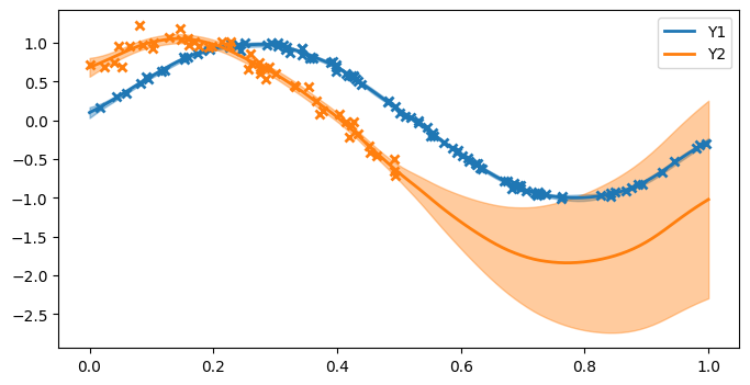
From the plots, we can see:

• The first function (blue) has low posterior variance everywhere because there are so many observations, and the noise variance is small.

• The second function (orange) has higher posterior variance near the data, because the data are more noisy, and very high posterior variance where there are no observations (x > 0.5).

• The model has done a reasonable job of estimating the noise variance and lengthscale.

• The model recognises the correlation between the two functions and is able to suggest (with uncertainty) that because x > 0.5 the orange curve should follow the blue curve (which we know to be the truth from the data-generating procedure).

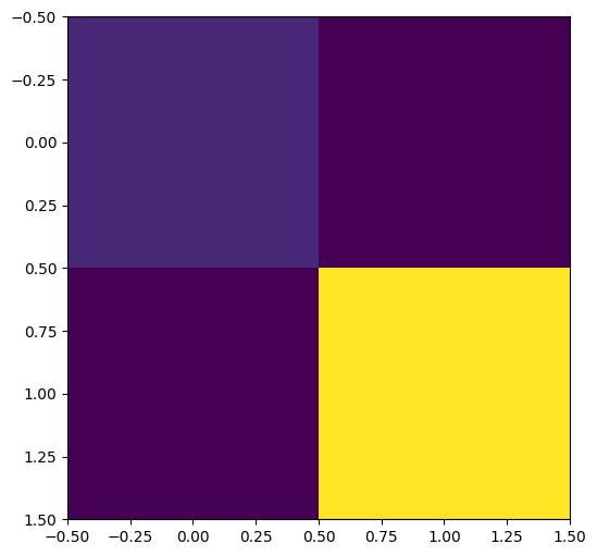
The covariance matrix between outputs is as follows:

B = coreg.output_covariance().numpy()
print("B =", B)
plt.imshow(B)

B = [[2.85339696 2.65481396]
 [2.65481396 4.44666954]]

References

Bonilla, Edwin V., Kian M. Chai, and Christopher Williams. “Multi-task Gaussian process prediction.” Advances in neural information processing systems. 2008.