Stochastic Variational Inference for scalability with SVGP

One of the main criticisms of Gaussian processes is their scalability to large datasets. In this notebook, we illustrate how to use the state-of-the-art Stochastic Variational Gaussian Process (SVGP) (Hensman, et. al. 2013) to overcome this problem.

%matplotlib inline
import itertools
import time

import matplotlib.pyplot as plt
import numpy as np
import tensorflow as tf

import gpflow
from gpflow.ci_utils import reduce_in_tests

plt.style.use("ggplot")

# for reproducibility of this notebook:
rng = np.random.RandomState(123)
tf.random.set_seed(42)

2024-02-07 11:45:55.903522: I external/local_tsl/tsl/cuda/cudart_stub.cc:31] Could not find cuda drivers on your machine, GPU will not be used.
2024-02-07 11:45:55.943839: E external/local_xla/xla/stream_executor/cuda/cuda_dnn.cc:9261] Unable to register cuDNN factory: Attempting to register factory for plugin cuDNN when one has already been registered
2024-02-07 11:45:55.943874: E external/local_xla/xla/stream_executor/cuda/cuda_fft.cc:607] Unable to register cuFFT factory: Attempting to register factory for plugin cuFFT when one has already been registered
2024-02-07 11:45:55.945128: E external/local_xla/xla/stream_executor/cuda/cuda_blas.cc:1515] Unable to register cuBLAS factory: Attempting to register factory for plugin cuBLAS when one has already been registered
2024-02-07 11:45:55.951720: I external/local_tsl/tsl/cuda/cudart_stub.cc:31] Could not find cuda drivers on your machine, GPU will not be used.
2024-02-07 11:45:55.952478: I tensorflow/core/platform/cpu_feature_guard.cc:182] This TensorFlow binary is optimized to use available CPU instructions in performance-critical operations.
To enable the following instructions: AVX2 AVX512F FMA, in other operations, rebuild TensorFlow with the appropriate compiler flags.

2024-02-07 11:45:56.952608: W tensorflow/compiler/tf2tensorrt/utils/py_utils.cc:38] TF-TRT Warning: Could not find TensorRT

Generating data

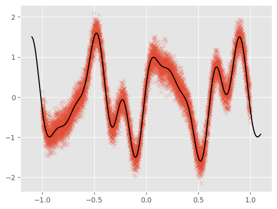
For this notebook example, we generate 10,000 noisy observations from a test function: \begin{equation} f(x) = \sin(3\pi x) + 0.3\cos(9\pi x) + \frac{\sin(7 \pi x)}{2} \end{equation}

def func(x):
    return (
        np.sin(x * 3 * 3.14)
        + 0.3 * np.cos(x * 9 * 3.14)
        + 0.5 * np.sin(x * 7 * 3.14)
    )


N = 10000  # Number of training observations

X = rng.rand(N, 1) * 2 - 1  # X values
Y = func(X) + 0.2 * rng.randn(N, 1)  # Noisy Y values
data = (X, Y)

We plot the data along with the noiseless generating function:

plt.plot(X, Y, "x", alpha=0.2)
Xt = np.linspace(-1.1, 1.1, 1000)[:, None]
Yt = func(Xt)
plt.plot(Xt, Yt, c="k")

Building the model

The main idea behind SVGP is to approximate the true GP posterior with a GP conditioned on a small set of “inducing” values. This smaller set can be thought of as summarizing the larger dataset. For this example, we will select a set of 50 inducing locations that are initialized from the training dataset:

M = 50  # Number of inducing locations

kernel = gpflow.kernels.SquaredExponential()
Z = X[
    :M, :
].copy()  # Initialize inducing locations to the first M inputs in the dataset

m = gpflow.models.SVGP(kernel, gpflow.likelihoods.Gaussian(), Z, num_data=N)

Likelihood computation: batch vs. minibatch

First we showcase the model’s performance using the whole dataset to compute the ELBO.

elbo = tf.function(m.elbo)

# TensorFlow re-traces & compiles a `tf.function`-wrapped method at *every* call if the arguments are numpy arrays instead of tf.Tensors. Hence:
tensor_data = tuple(map(tf.convert_to_tensor, data))
elbo(tensor_data)  # run it once to trace & compile

<tf.Tensor: shape=(), dtype=float64, numpy=-17730.676725310346>

%%timeit
elbo(tensor_data)

27 ms ± 5.72 ms per loop (mean ± std. dev. of 7 runs, 10 loops each)

We can speed up this calculation by using minibatches of the data. For this example, we use minibatches of size 100.

minibatch_size = 100

train_dataset = tf.data.Dataset.from_tensor_slices((X, Y)).repeat().shuffle(N)

train_iter = iter(train_dataset.batch(minibatch_size))

ground_truth = elbo(tensor_data).numpy()

%%timeit
elbo(next(train_iter))

1.34 ms ± 579 µs per loop (mean ± std. dev. of 7 runs, 1 loop each)

Stochastical estimation of ELBO

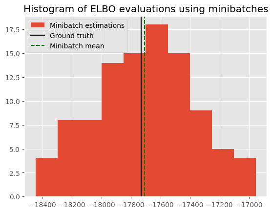
The minibatch estimate should be an unbiased estimator of the ground_truth. Here we show a histogram of the value from different evaluations, together with its mean and the ground truth. The small difference between the mean of the minibatch estimations and the ground truth shows that the minibatch estimator is working as expected.

evals = [
    elbo(minibatch).numpy() for minibatch in itertools.islice(train_iter, 100)
]

plt.hist(evals, label="Minibatch estimations")
plt.axvline(ground_truth, c="k", label="Ground truth")
plt.axvline(np.mean(evals), c="g", ls="--", label="Minibatch mean")
plt.legend()
plt.title("Histogram of ELBO evaluations using minibatches")
print(
    "Discrepancy between ground truth and minibatch estimate:",
    ground_truth - np.mean(evals),
)

Discrepancy between ground truth and minibatch estimate: -21.802624793072027

Minibatches speed up computation

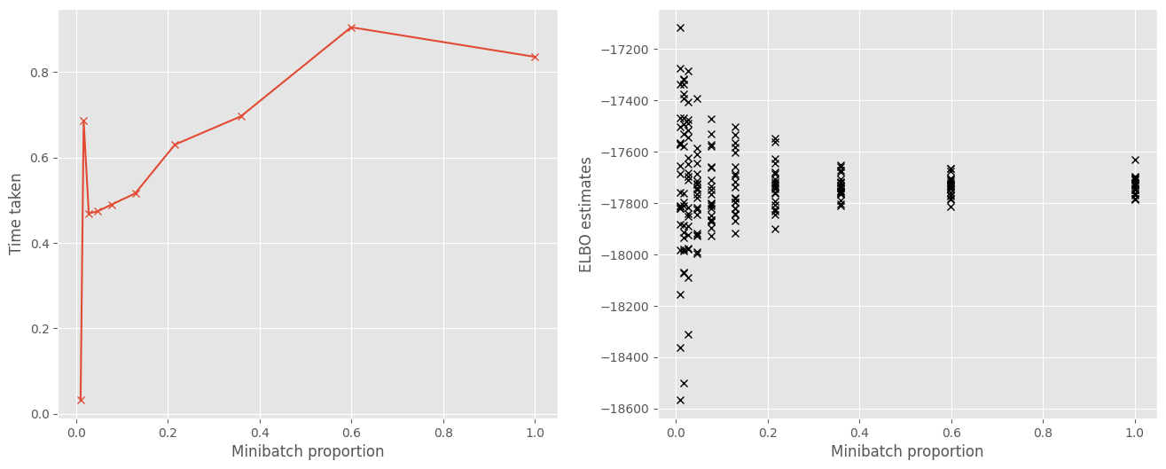
The reason for using minibatches is that it decreases the time needed to make an optimization step, because estimating the objective is computationally cheaper with fewer data points. Here we plot the change in time required with the size of the minibatch. We see that smaller minibatches result in a cheaper estimate of the objective.

# Evaluate objective for different minibatch sizes
minibatch_proportions = np.logspace(-2, 0, 10)
times = []
objs = []
for mbp in minibatch_proportions:
    batchsize = int(N * mbp)
    train_iter = iter(train_dataset.batch(batchsize))
    start_time = time.time()
    objs.append(
        [elbo(minibatch) for minibatch in itertools.islice(train_iter, 20)]
    )
    times.append(time.time() - start_time)

f, (ax1, ax2) = plt.subplots(1, 2, figsize=(16, 6))
ax1.plot(minibatch_proportions, times, "x-")
ax1.set_xlabel("Minibatch proportion")
ax1.set_ylabel("Time taken")

ax2.plot(minibatch_proportions, np.array(objs), "kx")
ax2.set_xlabel("Minibatch proportion")
ax2.set_ylabel("ELBO estimates")

Text(0, 0.5, 'ELBO estimates')

Running stochastic optimization

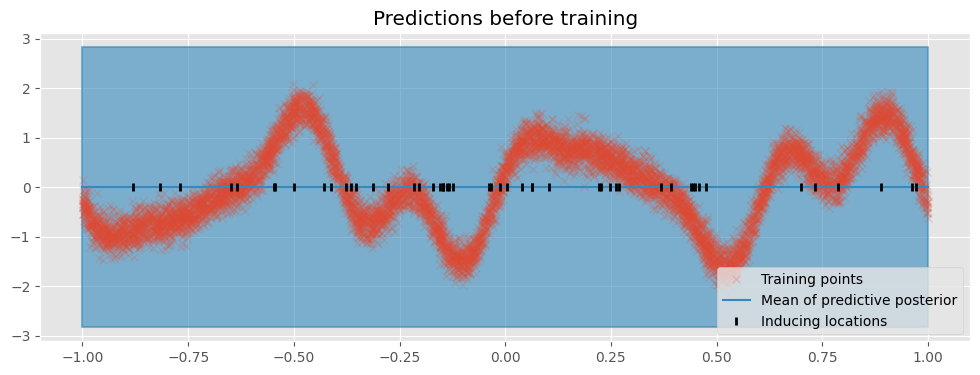
First we create a utility function that plots the model’s predictions:

def plot(title=""):
    plt.figure(figsize=(12, 4))
    plt.title(title)
    pX = np.linspace(-1, 1, 100)[:, None]  # Test locations
    pY, pYv = m.predict_y(pX)  # Predict Y values at test locations
    plt.plot(X, Y, "x", label="Training points", alpha=0.2)
    (line,) = plt.plot(pX, pY, lw=1.5, label="Mean of predictive posterior")
    col = line.get_color()
    plt.fill_between(
        pX[:, 0],
        (pY - 2 * pYv ** 0.5)[:, 0],
        (pY + 2 * pYv ** 0.5)[:, 0],
        color=col,
        alpha=0.6,
        lw=1.5,
    )
    Z = m.inducing_variable.Z.numpy()
    plt.plot(Z, np.zeros_like(Z), "k|", mew=2, label="Inducing locations")
    plt.legend(loc="lower right")


plot(title="Predictions before training")

Now we can train our model. For optimizing the ELBO, we use the Adam Optimizer (Kingma and Ba 2015) which is designed for stochastic objective functions. We create a run_adam utility function to perform the optimization.

minibatch_size = 100

# We turn off training for inducing point locations
gpflow.set_trainable(m.inducing_variable, False)


def run_adam(model, iterations):
    """
    Utility function running the Adam optimizer

    :param model: GPflow model
    :param interations: number of iterations
    """
    # Create an Adam Optimizer action
    logf = []
    train_iter = iter(train_dataset.batch(minibatch_size))
    training_loss = model.training_loss_closure(train_iter, compile=True)
    optimizer = tf.optimizers.Adam()

    @tf.function
    def optimization_step():
        optimizer.minimize(training_loss, model.trainable_variables)

    for step in range(iterations):
        optimization_step()
        if step % 10 == 0:
            elbo = -training_loss().numpy()
            logf.append(elbo)
    return logf

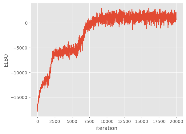
Now we run the optimization loop for 20,000 iterations.

maxiter = reduce_in_tests(20000)

logf = run_adam(m, maxiter)
plt.plot(np.arange(maxiter)[::10], logf)
plt.xlabel("iteration")
plt.ylabel("ELBO")

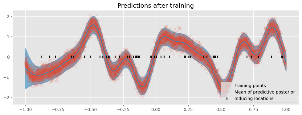
Finally, we plot the model’s predictions.

plot("Predictions after training")

Further reading

Several notebooks expand on this one:

• Advanced Sparse GP regression, which goes into deeper detail on sparse Gaussian process methods.

• Optimization discussing optimizing GP models.

• Natural gradients for optimizing SVGP models efficiently.

References:

Hensman, James, Nicolo Fusi, and Neil D. Lawrence. “Gaussian processes for big data.” Uncertainty in Artificial Intelligence (2013).

Kingma, Diederik P., and Jimmy Ba. “Adam: A method for stochastic optimization.” arXiv preprint arXiv:1412.6980 (2014).