Kernel Design

It’s easy to make new kernels in GPflow. To demonstrate, we’ll have a look at the Brownian motion kernel, whose function is \begin{equation} k(x, x') = \sigma^2 \text{min}(x, x') \end{equation} where \(\sigma^2\) is a variance parameter.

import matplotlib.pyplot as plt
import numpy as np
import tensorflow as tf

import gpflow
from gpflow.utilities import positive, print_summary

plt.style.use("ggplot")
%matplotlib inline

2024-02-07 11:46:53.033410: I external/local_tsl/tsl/cuda/cudart_stub.cc:31] Could not find cuda drivers on your machine, GPU will not be used.
2024-02-07 11:46:53.074767: E external/local_xla/xla/stream_executor/cuda/cuda_dnn.cc:9261] Unable to register cuDNN factory: Attempting to register factory for plugin cuDNN when one has already been registered
2024-02-07 11:46:53.074807: E external/local_xla/xla/stream_executor/cuda/cuda_fft.cc:607] Unable to register cuFFT factory: Attempting to register factory for plugin cuFFT when one has already been registered
2024-02-07 11:46:53.076192: E external/local_xla/xla/stream_executor/cuda/cuda_blas.cc:1515] Unable to register cuBLAS factory: Attempting to register factory for plugin cuBLAS when one has already been registered
2024-02-07 11:46:53.083065: I external/local_tsl/tsl/cuda/cudart_stub.cc:31] Could not find cuda drivers on your machine, GPU will not be used.
2024-02-07 11:46:53.083967: I tensorflow/core/platform/cpu_feature_guard.cc:182] This TensorFlow binary is optimized to use available CPU instructions in performance-critical operations.
To enable the following instructions: AVX2 AVX512F FMA, in other operations, rebuild TensorFlow with the appropriate compiler flags.

2024-02-07 11:46:54.152450: W tensorflow/compiler/tf2tensorrt/utils/py_utils.cc:38] TF-TRT Warning: Could not find TensorRT

To make this new kernel class, we inherit from the base class gpflow.kernels.Kernel and implement the three functions below. NOTE: Depending on the kernel to be implemented, other classes can be more adequate. For example, if the kernel to be implemented is isotropic stationary, you can immediately subclass gpflow.kernels.IsotropicStationary (at which point you only have to override K_r or K_r2; see the IsotropicStationary class docstring). Stationary but anisotropic kernels should subclass gpflow.kernels.AnisotropicStationary and override K_d.

__init__

In this simple example, the constructor takes no argument (though it could, if that was convenient, for example to pass in an initial value for variance). It must call the constructor of the superclass with appropriate arguments. Brownian motion is only defined in one dimension, and we’ll assume that the active_dims are [0], for simplicity.

We’ve added a parameter to the kernel using the Parameter class. Using this class lets the parameter be used in computing the kernel function, and it will automatically be recognised for optimization (or MCMC). Here, the variance parameter is initialized at 1, and constrained to be positive.

K

This is where you implement the kernel function itself. This takes two arguments, X and X2. By convention, we make the second argument optional (it defaults to None).

Inside K, all the computation must be done with TensorFlow - here we’ve used tf.minimum. When GPflow executes the K function, X and X2 will be TensorFlow tensors, and parameters such as self.variance behave like TensorFlow tensors as well.

K_diag

This convenience function allows GPflow to save memory at predict time. It’s simply the diagonal of the K function, in the case where X2 is None. It must return a one-dimensional vector, so we use TensorFlow’s reshape command.

class Brownian(gpflow.kernels.Kernel):
    def __init__(self):
        super().__init__(active_dims=[0])
        self.variance = gpflow.Parameter(1.0, transform=positive())

    def K(self, X, X2=None):
        if X2 is None:
            X2 = X
        return self.variance * tf.minimum(
            X, tf.transpose(X2)
        )  # this returns a 2D tensor

    def K_diag(self, X):
        return self.variance * tf.reshape(X, (-1,))  # this returns a 1D tensor


k_brownian = Brownian()
print_summary(k_brownian, fmt="notebook")

name	class	transform	prior	trainable	shape	dtype	value
Brownian.variance	Parameter	Softplus		True	()	float64	1

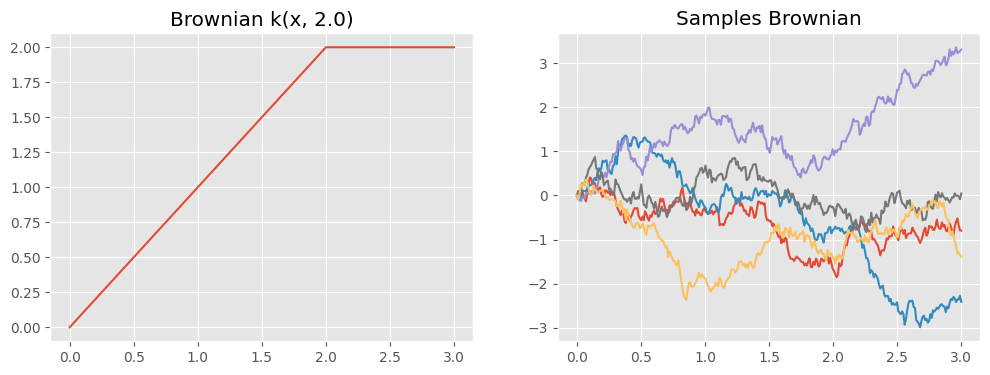
We can now evaluate our new kernel function and draw samples from a Gaussian process with this covariance:

np.random.seed(23)  # for reproducibility


def plotkernelsample(k, ax, xmin=0, xmax=3):
    xx = np.linspace(xmin, xmax, 300)[:, None]
    K = k(xx)
    ax.plot(xx, np.random.multivariate_normal(np.zeros(300), K, 5).T)
    ax.set_title("Samples " + k.__class__.__name__)


def plotkernelfunction(k, ax, xmin=0, xmax=3, other=0):
    xx = np.linspace(xmin, xmax, 100)[:, None]
    ax.plot(xx, k(xx, np.zeros((1, 1)) + other))
    ax.set_title(k.__class__.__name__ + " k(x, %.1f)" % other)


f, axes = plt.subplots(1, 2, figsize=(12, 4), sharex=True)
plotkernelfunction(k_brownian, axes[0], other=2.0)
plotkernelsample(k_brownian, axes[1])

Using the kernel in a model

Because we’ve inherited from the Kernel base class, this new kernel has all the properties needed to be used in GPflow. It also has some convenience features such as allowing the user to call

k(X, X2)

which computes the kernel matrix.

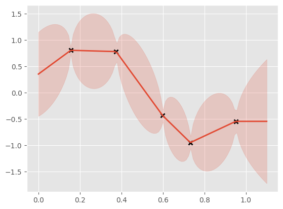
To show that this kernel works, let’s use it inside GP regression. We’ll see that Brownian motion has quite interesting properties. To add a little flexibility, we’ll add a Constant kernel to our Brownian kernel, and the GPR class will handle the noise.

np.random.seed(42)
X = np.random.rand(5, 1)
Y = np.sin(X * 6) + np.random.randn(*X.shape) * 0.001

k1 = Brownian()
k2 = gpflow.kernels.Constant()
k = k1 + k2

m = gpflow.models.GPR((X, Y), kernel=k)
# m.likelihood.variance.assign(1e-6)

opt = gpflow.optimizers.Scipy()
opt.minimize(m.training_loss, variables=m.trainable_variables)
print_summary(m, fmt="notebook")

xx = np.linspace(0, 1.1, 100).reshape(100, 1)
mean, var = m.predict_y(xx)
plt.plot(X, Y, "kx", mew=2)
(line,) = plt.plot(xx, mean, lw=2)
plt.fill_between(
    xx[:, 0],
    mean[:, 0] - 2 * np.sqrt(var[:, 0]),
    mean[:, 0] + 2 * np.sqrt(var[:, 0]),
    color=line.get_color(),
    alpha=0.2,
)

name	class	transform	prior	trainable	shape	dtype	value
GPR.kernel.kernels[0].variance	Parameter	Softplus		True	()	float64	2.33113
GPR.kernel.kernels[1].variance	Parameter	Softplus		True	()	float64	0.283867
GPR.likelihood.variance	Parameter	Softplus + Shift		True	()	float64	1.06518e-06

See also

For more details on how to manipulate existing kernels (or the one you just created!), please refer to the kernels notebook.