Manipulating kernels

GPflow comes with a range of kernels. In this notebook, we examine some of them, show how you can combine them to make new kernels, and discuss the active_dims feature.

import matplotlib.pyplot as plt
import numpy as np

import gpflow
from gpflow.ci_utils import reduce_in_tests

plt.style.use("ggplot")
%matplotlib inline

2022-10-13 08:52:46.625264: I tensorflow/core/platform/cpu_feature_guard.cc:193] This TensorFlow binary is optimized with oneAPI Deep Neural Network Library (oneDNN) to use the following CPU instructions in performance-critical operations:  AVX2 AVX512F FMA
To enable them in other operations, rebuild TensorFlow with the appropriate compiler flags.
2022-10-13 08:52:46.748144: W tensorflow/stream_executor/platform/default/dso_loader.cc:64] Could not load dynamic library 'libcudart.so.11.0'; dlerror: libcudart.so.11.0: cannot open shared object file: No such file or directory
2022-10-13 08:52:46.748166: I tensorflow/stream_executor/cuda/cudart_stub.cc:29] Ignore above cudart dlerror if you do not have a GPU set up on your machine.
2022-10-13 08:52:46.776904: E tensorflow/stream_executor/cuda/cuda_blas.cc:2981] Unable to register cuBLAS factory: Attempting to register factory for plugin cuBLAS when one has already been registered
2022-10-13 08:52:47.399647: W tensorflow/stream_executor/platform/default/dso_loader.cc:64] Could not load dynamic library 'libnvinfer.so.7'; dlerror: libnvinfer.so.7: cannot open shared object file: No such file or directory
2022-10-13 08:52:47.399710: W tensorflow/stream_executor/platform/default/dso_loader.cc:64] Could not load dynamic library 'libnvinfer_plugin.so.7'; dlerror: libnvinfer_plugin.so.7: cannot open shared object file: No such file or directory
2022-10-13 08:52:47.399719: W tensorflow/compiler/tf2tensorrt/utils/py_utils.cc:38] TF-TRT Warning: Cannot dlopen some TensorRT libraries. If you would like to use Nvidia GPU with TensorRT, please make sure the missing libraries mentioned above are installed properly.
/home/circleci/project/gpflow/experimental/utils.py:42: UserWarning: You're calling gpflow.experimental.check_shapes.decorator.check_shapes which is considered *experimental*. Expect: breaking changes, poor documentation, and bugs.
  warn(
/home/circleci/project/gpflow/experimental/utils.py:42: UserWarning: You're calling gpflow.experimental.check_shapes.inheritance.inherit_check_shapes which is considered *experimental*. Expect: breaking changes, poor documentation, and bugs.
  warn(

Standard kernels in GPflow

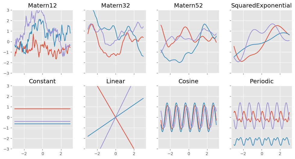
GPflow comes with lots of standard kernels. Some very simple kernels produce constant functions, linear functions, and white noise functions:

• gpflow.kernels.Constant

• gpflow.kernels.Linear

• gpflow.kernels.White

Some stationary functions produce samples with varying degrees of smoothness:

• gpflow.kernels.Exponential

• gpflow.kernels.Matern12

• gpflow.kernels.Matern32

• gpflow.kernels.Matern52

• gpflow.kernels.SquaredExponential (also known as gpflow.kernels.RBF)

• gpflow.kernels.RationalQuadratic

Two kernels produce periodic samples:

• gpflow.kernels.Cosine

• gpflow.kernels.Periodic

Other kernels that are implemented in core GPflow include:

• gpflow.kernels.Polynomial

• gpflow.kernels.ArcCosine (“neural network kernel”)

• gpflow.kernels.Coregion

Let’s define some plotting utils functions and have a look at samples from the prior for some of them:

def plotkernelsample(k, ax, xmin=-3, xmax=3):
    n_grid = reduce_in_tests(100)
    xx = np.linspace(xmin, xmax, n_grid)[:, None]
    K = k(xx)
    ax.plot(xx, np.random.multivariate_normal(np.zeros(n_grid), K, 3).T)
    ax.set_title(k.__class__.__name__)


np.random.seed(27)
f, axes = plt.subplots(2, 4, figsize=(12, 6), sharex=True, sharey=True)
plotkernelsample(gpflow.kernels.Matern12(), axes[0, 0])
plotkernelsample(gpflow.kernels.Matern32(), axes[0, 1])
plotkernelsample(gpflow.kernels.Matern52(), axes[0, 2])
plotkernelsample(gpflow.kernels.RBF(), axes[0, 3])
plotkernelsample(gpflow.kernels.Constant(), axes[1, 0])
plotkernelsample(gpflow.kernels.Linear(), axes[1, 1])
plotkernelsample(gpflow.kernels.Cosine(), axes[1, 2])
plotkernelsample(
    gpflow.kernels.Periodic(gpflow.kernels.SquaredExponential()), axes[1, 3]
)
_ = axes[0, 0].set_ylim(-3, 3)

/home/circleci/project/gpflow/experimental/utils.py:42: UserWarning: You're calling gpflow.experimental.check_shapes.checker.ShapeChecker.__init__ which is considered *experimental*. Expect: breaking changes, poor documentation, and bugs.
  warn(
2022-10-13 08:52:49.978212: W tensorflow/stream_executor/platform/default/dso_loader.cc:64] Could not load dynamic library 'libcuda.so.1'; dlerror: libcuda.so.1: cannot open shared object file: No such file or directory
2022-10-13 08:52:49.978497: W tensorflow/stream_executor/cuda/cuda_driver.cc:263] failed call to cuInit: UNKNOWN ERROR (303)
2022-10-13 08:52:49.978519: I tensorflow/stream_executor/cuda/cuda_diagnostics.cc:156] kernel driver does not appear to be running on this host (2b87543b4218): /proc/driver/nvidia/version does not exist
2022-10-13 08:52:49.979247: I tensorflow/core/platform/cpu_feature_guard.cc:193] This TensorFlow binary is optimized with oneAPI Deep Neural Network Library (oneDNN) to use the following CPU instructions in performance-critical operations:  AVX2 AVX512F FMA
To enable them in other operations, rebuild TensorFlow with the appropriate compiler flags.

First example: create a Matern 3/2 covariance kernel

Many kernels have hyperparameters, for example variance and lengthscales. You can change the value of these parameters from their default value of 1.0.

k = gpflow.kernels.Matern32(variance=10.0, lengthscales=2)

NOTE: The values specified for the variance and lengthscales parameters are floats.

To get information about the kernel, use print_summary(k) (plain text) or, in a notebook, pass the option fmt="notebook" to obtain a nicer rendering:

from gpflow.utilities import print_summary

print_summary(k)
print_summary(k, fmt="notebook")
# You can change the default format as follows:
gpflow.config.set_default_summary_fmt("notebook")
print_summary(k)

╒═══════════════════════╤═══════════╤═════════════╤═════════╤═════════════╤═════════╤═════════╤═════════╕
│ name                  │ class     │ transform   │ prior   │ trainable   │ shape   │ dtype   │   value │
╞═══════════════════════╪═══════════╪═════════════╪═════════╪═════════════╪═════════╪═════════╪═════════╡
│ Matern32.variance     │ Parameter │ Softplus    │         │ True        │ ()      │ float64 │      10 │
├───────────────────────┼───────────┼─────────────┼─────────┼─────────────┼─────────┼─────────┼─────────┤
│ Matern32.lengthscales │ Parameter │ Softplus    │         │ True        │ ()      │ float64 │       2 │
╘═══════════════════════╧═══════════╧═════════════╧═════════╧═════════════╧═════════╧═════════╧═════════╛

name	class	transform	prior	trainable	shape	dtype	value
Matern32.variance	Parameter	Softplus		True	()	float64	10
Matern32.lengthscales	Parameter	Softplus		True	()	float64	2

name	class	transform	prior	trainable	shape	dtype	value
Matern32.variance	Parameter	Softplus		True	()	float64	10
Matern32.lengthscales	Parameter	Softplus		True	()	float64	2

You can access the parameter values and assign new values with the same syntax as for models:

print(k.lengthscales)
k.lengthscales.assign(0.5)
print(k.lengthscales)

<Parameter: name=softplus, dtype=float64, shape=[], fn="softplus", numpy=2.0>
<Parameter: name=softplus, dtype=float64, shape=[], fn="softplus", numpy=0.5>

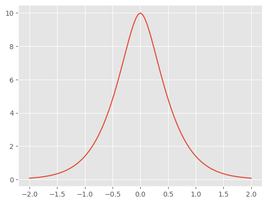
Finally, you can call the kernel object to compute covariance matrices:

X1 = np.array([[0.0]])
X2 = np.linspace(-2, 2, 101).reshape(-1, 1)

K21 = k(X2, X1)  # cov(f(X2), f(X1)): matrix with shape [101, 1]
K22 = k(
    X2
)  # equivalent to k(X2, X2) (but more efficient): matrix with shape [101, 101]

# plotting
plt.figure()
_ = plt.plot(X2, K21)

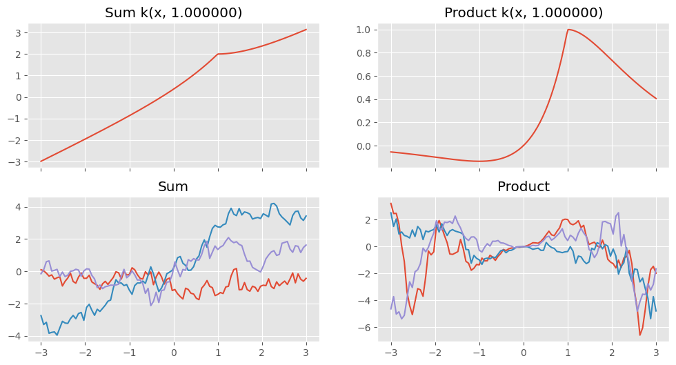
Combine kernels

Sums and products of kernels are also valid kernels. You can add or multiply instances of kernels to create a new composite kernel with the parameters of the old ones:

k1 = gpflow.kernels.Matern12()
k2 = gpflow.kernels.Linear()

k3 = k1 + k2
k4 = k1 * k2

print_summary(k3)
print_summary(k4)


def plotkernelfunction(k, ax, xmin=-3, xmax=3, other=0):
    n_grid = reduce_in_tests(200)
    xx = np.linspace(xmin, xmax, n_grid)[:, None]
    ax.plot(xx, k(xx, np.zeros((1, 1)) + other))
    ax.set_title(k.__class__.__name__ + " k(x, %f)" % other)


f, axes = plt.subplots(2, 2, figsize=(12, 6), sharex=True)
plotkernelfunction(k3, axes[0, 0], other=1.0)
plotkernelfunction(k4, axes[0, 1], other=1.0)
plotkernelsample(k3, axes[1, 0])
plotkernelsample(k4, axes[1, 1])

name	class	transform	prior	trainable	shape	dtype	value
Sum.kernels[0].variance	Parameter	Softplus		True	()	float64	1
Sum.kernels[0].lengthscales	Parameter	Softplus		True	()	float64	1
Sum.kernels[1].variance	Parameter	Softplus		True	()	float64	1

name	class	transform	prior	trainable	shape	dtype	value
Product.kernels[0].variance	Parameter	Softplus		True	()	float64	1
Product.kernels[0].lengthscales	Parameter	Softplus		True	()	float64	1
Product.kernels[1].variance	Parameter	Softplus		True	()	float64	1

Kernels for higher-dimensional input spaces

Kernels generalize to multiple dimensions straightforwardly. Stationary kernels support “Automatic Relevance Determination” (ARD), that is, having a different lengthscale parameter for each input dimension. Simply pass in an array of the same length as the number of input dimensions. NOTE: This means that the kernel object is then able to process only inputs of that dimension!

You can also initialize the lengthscales when the object is created:

k = gpflow.kernels.Matern52(lengthscales=[0.1, 0.2, 5.0])
print_summary(k)

name	class	transform	prior	trainable	shape	dtype	value
Matern52.variance	Parameter	Softplus		True	()	float64	1.0
Matern52.lengthscales	Parameter	Softplus		True	(3,)	float64	[0.1 0.2 5. ]

Specify active dimensions

When combining kernels, it’s often helpful to have bits of the kernel working on different dimensions. For example, to model a function that is linear in the first dimension and smooth in the second, we could use a combination of Linear and Matern52 kernels, one for each dimension.

To tell GPflow which dimension a kernel applies to, specify a list of integers as the value of the active_dims parameter.

k1 = gpflow.kernels.Linear(active_dims=[0])
k2 = gpflow.kernels.Matern52(active_dims=[1])
k = k1 + k2

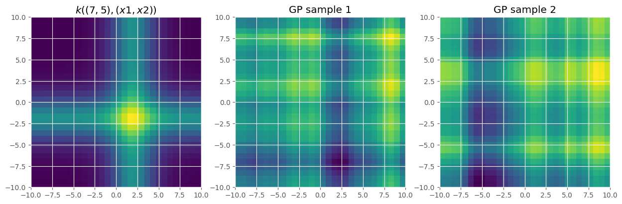
active_dims makes it easy to create additive models. Here we build an additive Matern 5/2 kernel:

k = gpflow.kernels.Matern52(
    active_dims=[0], lengthscales=2
) + gpflow.kernels.Matern52(active_dims=[1], lengthscales=2)

Let’s plot this kernel and sample from it:

n_grid = reduce_in_tests(30)
x = np.linspace(-10, 10, n_grid)
X, Y = np.meshgrid(x, x)
X = np.vstack((X.flatten(), Y.flatten())).T

x0 = np.array([[2.0, 2.0]])
# plot the kernel
KxX = k(X, x0).numpy().reshape(n_grid, n_grid)

fig, axes = plt.subplots(1, 3, figsize=(15, 5))
axes[0].imshow(KxX, extent=[-10, 10, -10, 10])
axes[0].set_title(f"$k((7, 5), (x1, x2))$")

# plot a GP sample
K = k(X).numpy()
Z = np.random.multivariate_normal(np.zeros(n_grid ** 2), K, 2)
axes[1].imshow(Z[0, :].reshape(n_grid, n_grid), extent=[-10, 10, -10, 10])
axes[1].set_title("GP sample 1")
axes[2].imshow(Z[1, :].reshape(n_grid, n_grid), extent=[-10, 10, -10, 10])
_ = axes[2].set_title("GP sample 2")

Define new covariance functions

GPflow makes it easy to define new covariance functions. See Kernel design for more information.